
In the process of three-dimensional composite crack propagation, the existing fracture criteria can not completely and accurately describe the crack propagation. In general engineering, most of them are the composite forms of mode I, II and III cracks, which means that the internal stress intensity factor K in the range of online elastic fracture mechanics is a very important parameter for the stage of crack fracture and stable propagation. The existence of mode II,III crack not only changes the size of the equivalent stress intensity factor, but also affects the crack propagation direction. The crack inclination is used to describe the influence of the existence of mode II and III cracks on the crack propagation direction.
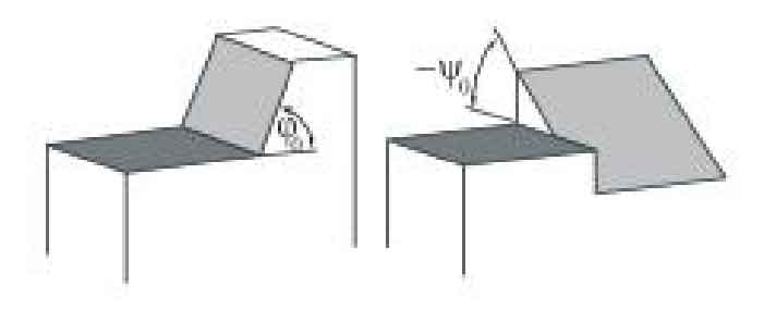
The definition of crack dip angle is based on the propagation direction of mode I crack. In mode I crack, the crack propagation direction is perpendicular to the stress direction; In the composite crack, due to the influence of Kii and kiII, the crack propagation direction will shift in the direction of pure mode I crack propagation. Crack dip angle is a parameter used to describe this offset degree. The definition diagram of crack dip angle is shown in Figure 1.
According to Richard criterion, the calculation formula of crack offset angle is given by the formula.
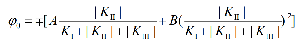
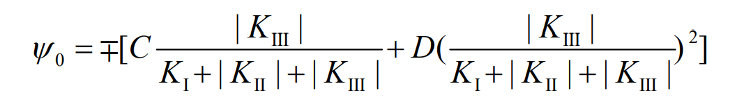


For the three-dimensional composite crack, it is very difficult to analyze the offset phenomenon of all nodes at the crack front in the propagation process. In order to explain the change trend of inclination angle in the crack propagation process under different distributed loads, the path for calculating the stress intensity factor in Figure 2 (i.e. the deepest crack) is selected in this section to study on this path, The change trend of crack propagation angle. The stress intensity factor of the deepest point of the crack is brought into the formula to obtain the change curve of crack Inclination under different loads, as shown in figures 3 and 4.
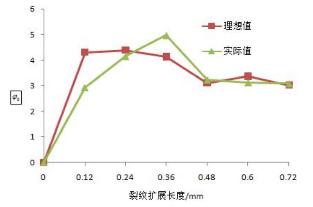
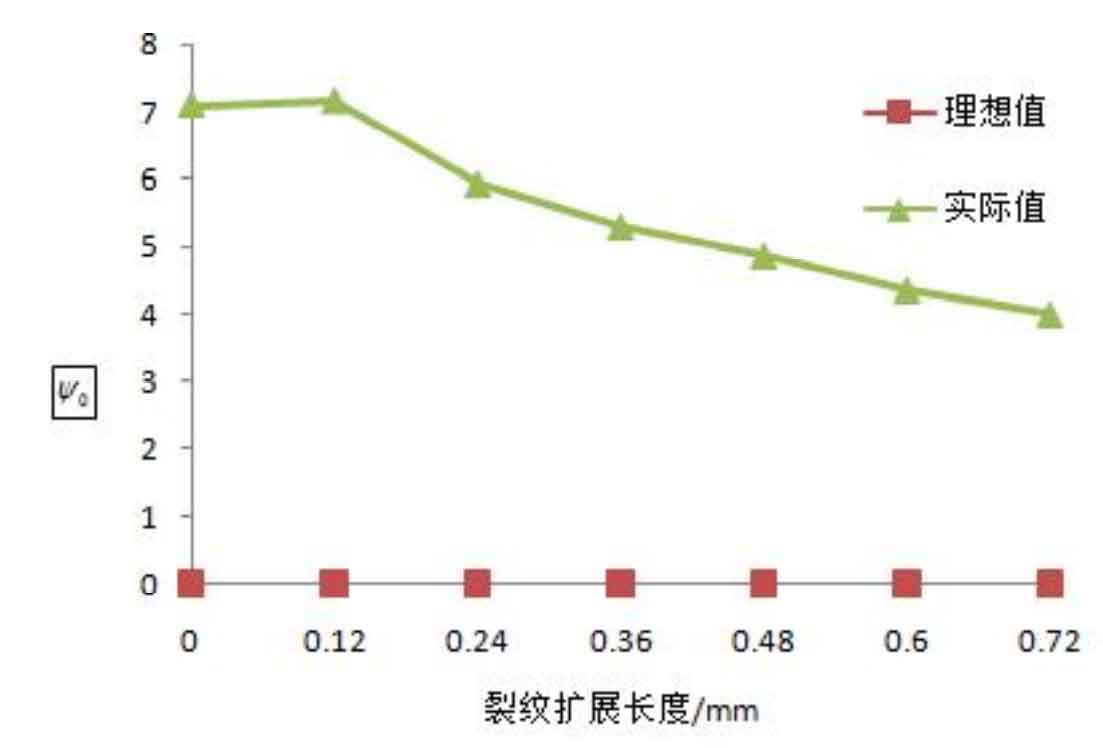
As can be seen from Fig. 4, in the stable crack growth stage, φ The change of 0 remains basically unchanged, and under the action of two different partial loads, φ The difference between the values of 0 is small, so the uneven load distribution pair can be obtained φ 0 has little effect. However, it can be seen from Fig. 4 that under different loads φ The 0 curve is very different; Under ideal uniform load φ 0 is almost zero, but under the action of actual load φ The value of 0 increases significantly.