
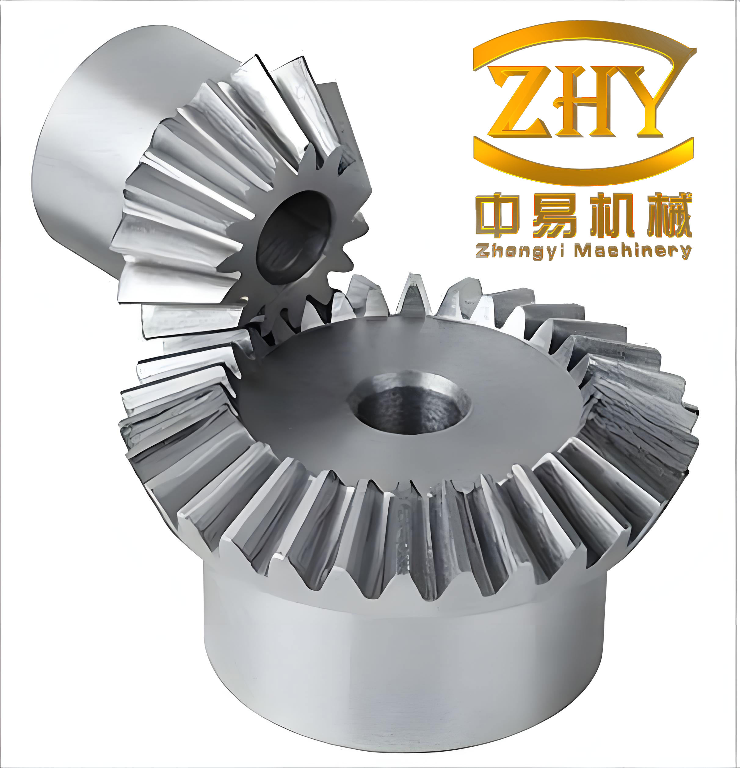
In the field of mechanical power transmission, straight bevel gears play a crucial role in applications requiring angular motion transfer between intersecting shafts. The accurate assessment of their bending strength is paramount for reliable design. However, traditional methods, which often simplify the three-dimensional problem into a two-dimensional one by assuming linear load distribution proportional to the distance from the cone apex, are inherently approximate. This simplification can lead to conservative or unsafe designs. Motivated by this limitation, we undertook a detailed investigation into the actual load distribution along the tooth contact line and the consequent root stress field in straight bevel gears. Our approach integrates an analytical formulation based on a compliance matrix method, three-dimensional finite element analysis (3D FEA), and three-dimensional photoelastic experimentation. This article presents our methodology, findings, and a critical comparison with conventional practices, aiming to provide a more precise foundation for the strength evaluation of straight bevel gears.
The core challenge in analyzing straight bevel gear tooth bending lies in determining the non-uniform load distribution along the spatially curved contact line. We developed a compliance matrix method to solve this. Consider an ideal meshing condition where two straight bevel gear teeth are in full contact along a line L. The normal load density function is q(ξ), where ξ is a coordinate along the contact line of length l. The normal deflection δi(ξ) at a point on gear i (i=1,2) can be related to the load distribution via an influence function integral:
$$ \delta_i(\xi) = \int_{0}^{l} C_i(\xi, \zeta) q(\zeta) d\zeta $$
where Ci(ξ, ζ) is the compliance function, representing the normal deflection at point ξ on gear i due to a unit normal force at point ζ. Under ideal contact, the composite normal deformation of the two teeth at any point must equal the displacement due to a presumed rigid body rotation of the gear pair, maintaining contact. This yields the compatibility condition:
$$ \delta_1(\xi) + \delta_2(\xi) = \theta r(\xi) $$
Here, θ is the small rigid rotation angle, and r(ξ) is the effective radius for normal displacement at point ξ. For discrete analysis, we divide the contact line into m nodes. The load density is approximated by concentrated forces Pj at these nodes (j=1,…,m). The deflections can then be expressed using a compliance matrix [C], where element Ckj is the normal deflection at node k due to a unit force at node j, summed for both gears. The discrete compatibility equation becomes:
$$ \sum_{j=1}^{m} C_{kj} P_j = \theta r_k \quad \text{for } k=1,…,m $$
We also have the equilibrium condition for the total normal load Fn:
$$ \sum_{j=1}^{m} P_j = F_n $$
Combining these, we obtain a system of m+1 equations with m+1 unknowns (P1,…, Pm, θ):
$$
\begin{bmatrix}
[C] & -\mathbf{r} \\
\mathbf{1}^T & 0
\end{bmatrix}
\begin{Bmatrix}
\mathbf{P} \\
\theta
\end{Bmatrix}
=
\begin{Bmatrix}
\mathbf{0} \\
F_n
\end{Bmatrix}
$$
where r is the vector of radii rk, and 1 is a row vector of ones. Solving this system yields the discrete load distribution P for the ideal contact case. For cases with initial contact gaps, a modified formulation incorporating gap closure deformations is used. This compliance matrix method forms the analytical backbone for predicting load distribution in straight bevel gears prior to stress analysis.
To apply this method and subsequently compute root stresses, we conducted detailed 3D finite element analysis. A model straight bevel gear pair with a transmission ratio of 1:1 was selected for study, allowing analysis of a single gear due to symmetry. The primary parameters of the model straight bevel gear are summarized in Table 1.
| Parameter | Symbol | Value | Unit |
|---|---|---|---|
| Number of Teeth | z | 20 | – |
| Module (at Large End) | m | 5 | mm |
| Pressure Angle | α | 20 | ° |
| Shaft Angle | Σ | 90 | ° |
| Face Width | b | 40 | mm |
| Pitch Cone Angle | δ | 45 | ° |
| Equivalent Radius at Mid-Face | rvm | 70.71 | mm |
A three-dimensional solid model of one tooth segment was created. The boundary conditions were simplified based on Saint-Venant’s principle. The model was constrained on the lateral boundaries (approximately one base pitch from the tooth center) and the lower boundary (about 1.5 times the module below the root circle) to approximate fixed support. The finite element mesh was generated using 20-node quadratic brick elements (SOLID95 in ANSYS terminology). The mesh was refined in the root fillet region where high stress gradients are expected, and coarser elsewhere. The final mesh comprised approximately 15,000 nodes and 3,500 elements. The tooth volume was longitudinally divided into 10 equal layers along the face width for detailed stress sampling. The contact line for any meshing position was discretized into 10 points corresponding to these layers.
The compliance coefficients Ckj were computed by applying a unit normal force at each of the 10 discrete contact points in turn and solving for the normal displacements at all points using the FEA solver. This process built the 10×10 compliance matrix [C] for each meshing position. Three characteristic meshing positions were analyzed: (a) tooth tip engagement, (b) the highest point of single tooth contact (HPSTC), and (c) a position near the root. For each case, assuming a total normal load Fn = 1000 N, the compliance matrix equation was solved to obtain the load distribution Pj. The results are presented in Table 2.
| Point (Layer) | Tooth Tip | HPSTC | Near Root |
|---|---|---|---|
| 1 (Large End) | 142.5 | 128.3 | 118.7 |
| 2 | 135.1 | 121.9 | 113.5 |
| 3 | 125.8 | 115.8 | 108.9 |
| 4 | 115.2 | 109.2 | 104.5 |
| 5 (Mid-Face) | 104.1 | 102.5 | 100.2 |
| 6 | 93.2 | 96.1 | 96.0 |
| 7 | 83.2 | 90.0 | 92.0 |
| 8 | 74.6 | 84.2 | 88.3 |
| 9 | 68.1 | 79.1 | 85.0 |
| 10 (Small End) | 64.2 | 74.9 | 82.9 |
The load distribution profiles, obtained by converting discrete forces to equivalent distributed loads, are plotted conceptually. They reveal a non-linear pattern decreasing from the large end to the small end, with a slight saddle-shaped fluctuation, especially for contact lines closer to the tip. This contradicts the traditional linear assumption. The load distribution for the straight bevel gear is inherently three-dimensional and influenced by the varying stiffness along the tooth.
With the calculated load distributions for each meshing position, a subsequent FEA run was performed applying these precise nodal forces as boundary conditions on the tooth flank. The maximum principal stress (tensile) and minimum principal stress (compressive) at the root fillet were extracted for each of the 10 longitudinal layers. The results for the most critical meshing position, the HPSTC, are shown in Table 3. The stress distribution across the face width exhibits a “drum-shaped” profile, with the peak tensile stress occurring near the large end (around layer 2 or 3), not at the mid-face as often assumed in traditional methods based on the equivalent spur gear. The stress decays towards the small end.
| Layer Number (1=Large End) | Max Tensile Stress (σt) | Max Compressive Stress (σc) |
|---|---|---|
| 1 | 58.2 | -49.8 |
| 2 | 62.7 | -53.1 |
| 3 | 61.9 | -52.4 |
| 4 | 58.5 | -50.0 |
| 5 | 53.8 | -46.5 |
| 6 | 48.5 | -42.3 |
| 7 | 43.1 | -37.9 |
| 8 | 38.0 | -33.8 |
| 9 | 33.6 | -30.2 |
| 10 | 30.1 | -27.3 |
To validate the numerical findings, a three-dimensional photoelastic experiment was conducted on a scaled-up epoxy resin model of the same straight bevel gear pair. The model geometry was scaled by a factor of 2 for manufacturing convenience. A specially designed loading fixture allowed precise positioning of the gears to achieve meshing at the HPSTC under near-ideal full-line contact. The model assembly was stress-frozen in a temperature-controlled oven under a carefully calibrated load. After freezing, the gear of interest was sliced into thin sections approximately parallel to the tooth axis, corresponding to the longitudinal layers in the FEA model. Each slice was analyzed using a transmission polariscope equipped with a digital compensator. The stress-optic law, combined with the oblique incidence method (using one normal and two oblique incidence measurements at ±30°), allowed determination of the individual stress components at critical points on the root fillet—specifically the points of maximum tensile and compressive stress in each slice.
The photoelastic results for the maximum tensile and compressive stresses along the face width are summarized in Table 4. The data conversion used the material fringe value fσ obtained from a calibration disk: fσ = 12.5 N/(mm·fringe). The stress at a point is given by:
$$ \sigma = \frac{n f_{\sigma}}{t} $$
where n is the measured fringe order and t is slice thickness. For 3D analysis, the oblique incidence method resolves the stress components. The principal stress difference is obtained from normal incidence: σ1 – σ3 = n0 fσ/t. Oblique measurements provide additional equations to solve for individual stresses. The detailed formulas used are:
$$ \sigma_x = \frac{f_{\sigma}}{t} \left[ n_0 – \frac{1}{\sin^2 \phi} (n_{+\phi} + n_{-\phi} – 2n_0 \cos \phi) \right] $$
$$ \tau_{xz} = \frac{f_{\sigma}}{2t \sin \phi} (n_{+\phi} – n_{-\phi}) $$
where φ is the oblique angle (30°), and n0, n+φ, n-φ are fringe orders for normal and oblique incidences, respectively. The maximum principal stresses were then derived.
| Slice (≈Layer) | Max Tensile Stress (σt) | Max Compressive Stress (σc) |
|---|---|---|
| 1 (Large End) | 55.1 | -47.2 |
| 2 | 60.3 | -50.8 |
| 3 | 59.5 | -49.9 |
| 4 | 56.0 | -47.5 |
| 5 | 51.6 | -44.0 |
| 6 | 46.5 | -39.8 |
| 7 | 41.4 | -35.7 |
| 8 | 36.8 | -32.1 |
| 9 | 32.9 | -28.9 |
| 10 (Small End) | 29.0 | -25.8 |
A direct comparison between the FEA and photoelastic stress results for the straight bevel gear at HPSTC is graphically represented. The agreement is excellent for the central layers (2 to 9). Slight discrepancies at the extreme ends (layers 1 and 10) are attributed to minor imperfections in achieving perfect contact at the very ends of the tooth face width in the physical photoelastic model, a common challenge in experimental setups. The peak tensile stress from FEA is 62.7 MPa at layer 2, while photoelastic gives 60.3 MPa, a relative difference of about 3.8%. This close correlation validates the accuracy of the combined compliance matrix and FEA methodology for analyzing straight bevel gears.
The significance of these findings becomes apparent when contrasted with traditional straight bevel gear bending stress formulas. A widely used method calculates stress based on the equivalent spur gear at the mid-face width, applying the Lewis formula with a linear load distribution assumption. For our model straight bevel gear parameters and load, this traditional method yields a calculated root bending stress of approximately:
$$ \sigma_{traditional} = \frac{F_t}{b m_n Y} K_A K_V K_m $$
where Ft is the tangential force at the mid-face, b is face width, mn is normal module, Y is the Lewis form factor for the equivalent spur gear, and K factors are application, dynamic, and load distribution factors. Using typical values, the estimate ranges from 70 to 80 MPa for our loading condition. This is substantially higher (about 12-27%) than both the FEA peak of 62.7 MPa and the photoelastic peak of 60.3 MPa. This overestimation by the traditional method confirms that it is conservative but potentially leads to over-designed, heavier straight bevel gear drives. Our detailed 3D analysis reveals the actual load-sharing and stress distribution, enabling more efficient and accurate design optimization for straight bevel gears.
Further discussion on the load distribution mechanism in straight bevel gears is warranted. The compliance of a straight bevel gear tooth varies along its face width due to the changing cross-section and the cantilever effect relative to the gear blank. The large end, being wider and having a shorter effective cantilever length to the constrained root area, is generally stiffer. However, the kinematic condition of rigid body rotation during meshing forces a deformation pattern that must be accommodated by the elastic deflection. Our compliance matrix solution inherently captures this interaction. The resulting load is higher at the stiffer large end because to achieve the same imposed displacement (from rotation), a larger force is required at a stiffer point. The slight mid-face dip in load for some meshing positions may be related to the complex 3D bending and shear coupling effects. This nuanced behavior cannot be captured by a simple linear assumption. Understanding this is critical for designing straight bevel gears for high-performance applications where weight and size are constraints.
The implications for fatigue life prediction are also important. The location of the maximum stress near the large end, rather than uniformly distributed, suggests that fatigue cracks in straight bevel gears are more likely to initiate from this region. Traditional safety factors based on mid-face stress might be misleading. A more reliable fatigue analysis for straight bevel gears should use the actual stress gradient obtained from 3D methods like the one presented here. Furthermore, the load distribution results can inform the design of profile and lead modifications to optimize contact patterns and reduce peak stresses in straight bevel gears, enhancing their durability and load capacity.
In conclusion, our integrated investigation employing compliance matrix theory, three-dimensional finite element analysis, and three-dimensional photoelasticity has provided deep insights into the mechanical behavior of straight bevel gears. The key findings are: Firstly, the load distribution along the contact line of a straight bevel gear under ideal meshing is non-linear, decreasing from the large end to the small end with a characteristic fluctuation, deviating significantly from the simplistic linear model. Secondly, the consequent root stress distribution exhibits a drum-shaped profile across the face width, with the peak tensile stress consistently located near the large end of the straight bevel gear tooth. Thirdly, the excellent agreement between the numerical FEA results and the experimental photoelastic data validates the proposed analytical-numerical framework as a reliable tool for straight bevel gear analysis. Finally, comparison with traditional calculation methods confirms that those methods tend to overestimate the bending stress in straight bevel gears, leading to conservative designs. This work establishes a more accurate foundation for the strength evaluation and optimal design of straight bevel gears, potentially contributing to lighter, more efficient gear transmissions. Future work could extend this approach to spiral bevel gears and incorporate dynamic loading conditions for a comprehensive understanding of gear performance.