
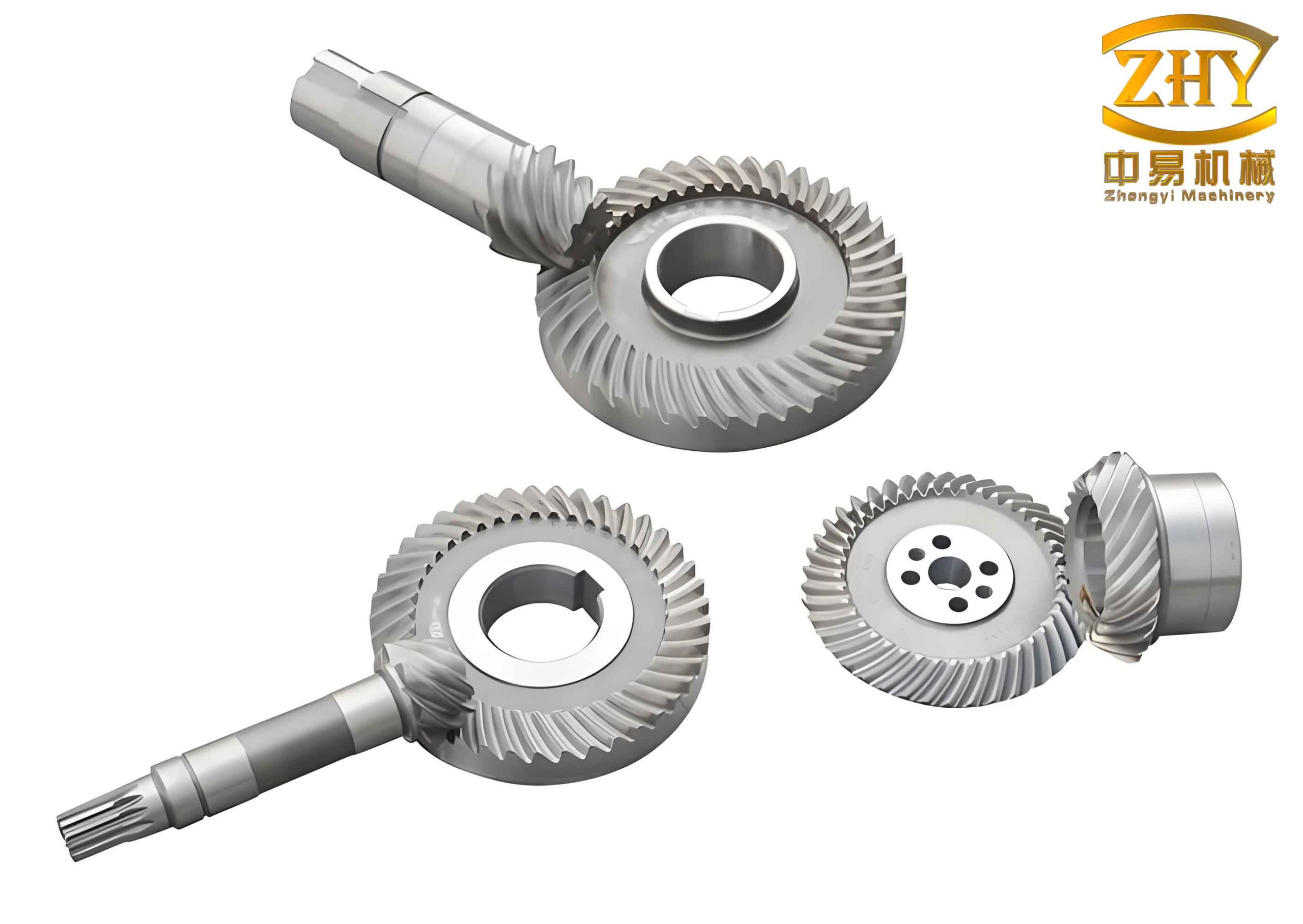
The pursuit of optimal performance, durability, and noise-vibration-harshness (NVH) characteristics in automotive powertrains has placed significant emphasis on the design and analysis of critical components such as hypoid or hyperboloidal gear sets. As a mainstay in automotive drive axles, hyperboloidal gears facilitate efficient power transfer between non-intersecting, non-parallel shafts, offering advantages like high load capacity, smooth operation, and the ability to achieve a lower center of gravity in vehicles. Accurately predicting their meshing behavior, particularly the loaded tooth contact pattern (LTCA), is paramount for ensuring performance and longevity. This article presents a detailed methodology for the contact analysis of automotive drive axle hyperboloidal gears, fusing the precision of analytical methods with the robust simulation capabilities of the finite element method (FEM). We establish the mathematical foundation for gear generation, derive tooth surface equations, compute transmission error analytically, and subsequently employ finite element analysis to visualize and evaluate three-dimensional contact patterns under load, validated against experimental results.
1. Mathematical Modeling of Hyperboloidal Gear Generation via the HFT Method
The formulation of an accurate tooth surface model is the cornerstone of any gear contact analysis. The Helical Formate Tool (HFT) method, a prevalent machining technique for hyperboloidal gears, serves as the basis for our mathematical model. The process begins with defining the cutter coordinate system. For a face-milling cutter, the coordinate system \( S_t(X_t, Y_t, Z_t) \) is fixed to the cutter head. The position vectors for points on the inner (\(G_g\)) and outer (\(G_p\)) blade edges are defined as follows, where \(r_g\) and \(r_p\) are the point radii, \(\alpha_g\) and \(\alpha_p\) are the blade pressure angles (positive for inner, negative for outer), and \(u_g\), \(u_p\), \(\theta_g\), \(\theta_p\) are surface parameters.
The vector equation for a point on the cutter surface and its corresponding unit normal vector in \(S_t\) are given by:
$$
\mathbf{r}_t^k(u_k, \theta_k) = \begin{bmatrix}
(r_k + u_k \sin \alpha_k) \cos \theta_k \\
(r_k + u_k \sin \alpha_k) \sin \theta_k \\
-u_k \cos \alpha_k \\
1
\end{bmatrix}, \quad k = g, p
$$
$$
\mathbf{n}_t^k(u_k, \theta_k) = [-\cos \alpha_k \cos \theta_k, \ -\cos \alpha_k \sin \theta_k, \ \sin \alpha_k]^T
$$
Next, the complex relative motion between the cutter and the workpiece during the HFT process is modeled. A series of coordinate transformations link the cutter system \(S_t\) to the machine frame \(S_m\), the cradle system \(S_c\), and finally to the workpiece (pinion) system \(S_1\). Key machine settings include the cutter tilt angle \(j\), swivel angle \(i\), angular position \(q_1\), radial distance \(S_{r1}\), machine center to back \(E_{m1}\), sliding base \(X_b\), offset \(X_{p1}\), and the work head rotation angle \(\gamma_m\). The generating motion is defined by the ratio \(R_b\), relating the cradle rotation \(\phi\) to the workpiece rotation \(\psi\) (\(\phi = R_b \psi\)).
Applying these coordinate transformations, the pinion tooth surface equation \(\mathbf{r}_1\) and its unit normal \(\mathbf{n}_1\) in the pinion coordinate system are derived:
$$
\mathbf{r}_1(u_k, \theta_k, \psi) = \mathbf{M}_{1d} \mathbf{M}_{dh} \mathbf{M}_{hs} \mathbf{M}_{sm} \mathbf{M}_{mc} \mathbf{M}_{cj} \mathbf{M}_{jt} \mathbf{r}_t^k(u_k, \theta_k)
$$
$$
\mathbf{n}_1(u_k, \theta_k, \psi) = \mathbf{L}_{1d} \mathbf{L}_{dh} \mathbf{L}_{hs} \mathbf{L}_{sm} \mathbf{L}_{mc} \mathbf{L}_{cj} \mathbf{L}_{jt} \mathbf{n}_t^k(u_k, \theta_k)
$$
Here, \(\mathbf{M}_{ij}\) are the homogeneous transformation matrices, and \(\mathbf{L}_{ij}\) are the corresponding \(3 \times 3\) rotation matrices extracted from them. For the gear (wheel), which is typically generated by a formate (non-generating) process, the model simplifies. This is a special case of the HFT model with parameters set to zero: \(j=0\), \(X_b=0\), \(E_{m1}=0\), \(R_b=0\), \(\phi=0\), and \(\psi=0\). Applying these conditions yields the gear tooth surface equations \(\mathbf{r}_2\) and \(\mathbf{n}_2\).
2. Analytical Determination of Transmission Error (TCA)
Tooth Contact Analysis (TCA) mathematically simulates the meshing process of a gear pair. For hyperboloidal gears with a 90-degree shaft angle and an offset \(\Delta E\), the meshing condition dictates that at any point of contact, the position vectors and surface normals of both tooth surfaces, expressed in a fixed global coordinate system \(S_a\), must coincide.
The transformed pinion and gear surfaces in \(S_a\) are:
$$
\mathbf{r}_a^1(u_1, \theta_1, \phi_1) = \mathbf{M}_{ad} \mathbf{M}_{d1} \mathbf{r}_1(u_1, \theta_1)
$$
$$
\mathbf{r}_a^2(u_2, \theta_2, \phi_2) = \mathbf{M}_{ab} \mathbf{M}_{b2} \mathbf{r}_2(u_2, \theta_2)
$$
$$
\mathbf{n}_a^1(u_1, \theta_1, \phi_1) = \mathbf{L}_{ad} \mathbf{L}_{d1} \mathbf{n}_1(u_1, \theta_1)
$$
$$
\mathbf{n}_a^2(u_2, \theta_2, \phi_2) = \mathbf{L}_{ab} \mathbf{L}_{b2} \mathbf{n}_2(u_2, \theta_2)
$$
The conditions for continuous tangency are:
$$
\mathbf{r}_a^1(u_1, \theta_1, \phi_1) = \mathbf{r}_a^2(u_2, \theta_2, \phi_2)
$$
$$
\mathbf{n}_a^1(u_1, \theta_1, \phi_1) = \mathbf{n}_a^2(u_2, \theta_2, \phi_2)
$$
This system yields five independent scalar equations with six unknowns \((u_1, \theta_1, u_2, \theta_2, \phi_1, \phi_2)\). By prescribing the pinion rotation angle \(\phi_1\) as an input, the system can be solved iteratively to find the corresponding contact point parameters. Tracing these points across the path of contact provides the meshing sequence. The transmission error, a critical indicator of meshing smoothness and noise excitation, is then calculated as the deviation from perfect conjugate motion:
$$
\Delta \phi_2(\phi_1) = \left( \phi_2 – \phi_2^{(0)} \right) – \frac{z_1}{z_2} \left( \phi_1 – \phi_1^{(0)} \right)
$$
where \(z_1\) and \(z_2\) are the numbers of teeth, and \(\phi_1^{(0)}, \phi_2^{(0)}\) are the initial contact angles at a reference point.
3. Numerical Tooth Surface Generation and 3D Modeling
For finite element analysis, a discrete 3D solid model of the hyperboloidal gears is required. The analytical surface equations \(\mathbf{r}_1\) and \(\mathbf{r}_2\) are evaluated over a grid of parameters \((u, \theta)\) to generate dense point clouds representing the active tooth flanks. These points are then processed using CAD software (e.g., Siemens NX or similar) to construct B-rep or parametric solid models of the complete pinion and gear. To facilitate high-quality hexahedral meshing in the subsequent FEM step, the model of a single tooth is often segmented using auxiliary surfaces and exported in a neutral format like Parasolid (.x_t).
4. Finite Element Simulation for Loaded Tooth Contact Analysis
The finite element method transcends the limitations of classical Hertzian contact theory for hyperboloidal gears, which involves complex curvature calculations and may yield anomalous results. FEM directly simulates the deformation under load, providing a realistic, three-dimensional visualization of the contact zone. The workflow within a commercial FEA package like ABAQUS involves three main stages: Pre-processing, Solution, and Post-processing.
The pre-processing stage involves importing the gear geometry, defining material properties (density \(\rho\), Young’s modulus \(E\), Poisson’s ratio \(\nu\)), and creating the assembly. A critical step is meshing; the segmented tooth model allows for the creation of a structured hexahedral mesh, which is generally more accurate and efficient for contact problems than tetrahedral meshes. Surface-to-surface contact pairs are defined between the pinion and gear teeth, with appropriate friction properties.
The solution phase involves applying boundary conditions and loads. The pinion and gear shafts are constrained appropriately (e.g., coupling reference points), and a static torque \(T\) is applied to the pinion to simulate the driving condition. A static, general step is used for the solver.
The post-processing stage yields the field outputs, most importantly the contact pressure distribution on the tooth flanks. The instantaneous contact ellipse at any given angular position manifests as the region of high contact stress. To construct the complete 3D contact pattern—which is the envelope of all instantaneous contact ellipses throughout the mesh cycle—a custom Python script is employed. The script operates as follows:
- Open the output database (.odb) and read the contact stress field output for all frames (increments).
- For each element on the contact surface, identify the maximum contact stress value it experiences across all frames.
- Write these maximum values for all elements to a new data file.
- In the visualization module, plotting this “maximum-over-time” contact stress field on the undeformed tooth shape reveals the full 3D contact pattern, effectively overlaying all transient ellipses onto a single image.
5. Case Study: Analysis of an Automotive Drive Axle Hyperboloidal Gear Set
To demonstrate the efficacy of the fused analytical-FEM approach, a case study of an automotive drive axle hyperboloidal gear pair is presented. The key geometric parameters are summarized in Table 1, and the HFT machine settings are listed in Table 2.
| Parameter | Pinion | Gear |
|---|---|---|
| Number of Teeth | 8 | 39 |
| Hand of Spiral | Left | Right |
| Shaft Angle | 90° | |
| Offset | 35 mm (below) | |
| Module (at Ref. Point) | 6.283 mm | |
| Spiral Angle (at Ref. Point) | 50.24° | 31.37° |
| Pressure Angle | 22.5° | |
| Face Width | 44.4 mm | 38 mm |
| Whole Depth | 12.15 mm | 11.89 mm |
| Parameter | Pinion (Convex) | Gear (Concave) |
|---|---|---|
| Cutter Radius | 120.91 mm | 115.86 mm |
| Blade Pressure Angle | -14° | -22.5° |
| Cutter Tilt Angle \(j\) | 12.11° | 0° |
| Cutter Swivel Angle \(i\) | 331.83° | 0° |
| Radial Setting \(S_r\) | 104.3279 mm | 109.058 mm |
| Angular Setting \(q\) | 83.21° | 67.845° |
| Machine Root Angle \(\gamma_m\) | 359.4° | 69.79° |
First, the transmission error was computed analytically using the derived TCA equations implemented in MATLAB. The resulting curve showed an amplitude of approximately 28 μrad. This result was cross-verified against a commercial gear design software (Gleason CAGE), which yielded a nearly identical amplitude of 28.5 μrad, validating the correctness of the analytical meshing model for these hyperboloidal gears.
Following the modeling workflow, a 3D solid model was created and imported into ABAQUS. After defining material properties (steel), applying a hexahedral mesh, setting up surface-to-surface contact, and applying boundary conditions and torque, a static analysis was performed. The Python script was executed to extract the maximum contact stress over the entire meshing cycle. The resulting 3D contact pattern on the gear concave flank is displayed as a contour plot.
For further validation, the same gear design was modeled in the dedicated gear analysis software MASTA. Under comparable load conditions, MASTA predicted a contact pattern strikingly similar in location, shape (inner-biased), and size to the pattern obtained from our ABAQUS simulation. This concordance strongly supports the accuracy of the proposed FEM-based contact analysis methodology for hyperboloidal gears.
Finally, experimental validation was conducted. The gear set was manufactured on a hypoid grinder using the parameters from Table 2. After grinding and careful measurement to ensure conformance to the design surface, the pair was tested on a Gleason T50 roll tester under a light load of 40 N·m. The observed contact pattern on the gear tooth closely matched both the FEM and MASTA predictions in terms of its central, slightly diagonal orientation and overall geometry, providing conclusive experimental proof of the method’s validity and practical utility for the design and analysis of hyperboloidal gears.
6. Conclusion
This article has detailed a comprehensive methodology for the contact analysis of hyperboloidal gears, synergistically combining analytical and finite element techniques. The analytical foundation provides a precise mathematical model for tooth generation and enables efficient calculation of fundamental kinematic performance metrics like transmission error. The finite element analysis builds upon this foundation to deliver a high-fidelity, three-dimensional simulation of the loaded contact pattern, overcoming the complexities and potential inaccuracies associated with purely analytical contact ellipse calculations. The complete workflow—from mathematical modeling and numerical surface generation to FEM simulation and automated result processing—was demonstrated through a practical automotive gear case study. The strong agreement between the FEM results, commercial software predictions, and physical roll test experiments confirms the correctness, feasibility, and engineering value of this fused approach. It provides gear engineers with a powerful and reliable tool for optimizing the contact characteristics and performance of critical hyperboloidal gear drives.