
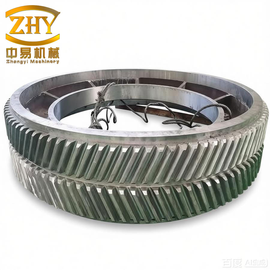
Herringbone gears are widely adopted in heavy-duty transmission systems such as marine propulsion, aerospace actuation, and high-power energy equipment because of their excellent load-carrying capacity, smooth meshing behavior, and negligible axial thrust. In my research, I focused on the contact fatigue performance of herringbone gears under manufacturing and assembly errors. The presence of centring error and angular misalignment can significantly alter the load distribution between the two mirrored helical gear halves, thereby increasing the risk of premature surface pitting. To address this challenge, I developed a systematic methodology that integrates finite element contact analysis, critical plane-based multiaxial fatigue life prediction, and an analytical eccentric load coefficient model. This article summarizes my master’s thesis work, with particular emphasis on the calculation framework, the influence of errors on gear life, and the practical implications for engineering design.
1. Introduction and Research Context
In modern mechanical transmission systems, gears must operate under increasingly demanding conditions of speed, torque, and reliability. Among various gear types, herringbone gears stand out due to their ability to eliminate axial forces while providing high torque density. However, their complex geometry makes them susceptible to manufacturing deviations and installation inaccuracies. A typical herringbone gear is formed by joining two helical gears with opposite helix angles, separated by a central gap known as the withdrawal groove. Ideal manufacturing would produce perfectly symmetric halves, but in practice, the two sides are often machined in separate setups, leading to a centring error δce. Additionally, the relatively large face width of herringbone gears makes them sensitive to angular misalignment during assembly. These errors cause uneven load sharing between the left and right helical gear halves, which elevates the local contact stress and reduces the fatigue life of the gear pair.
The primary objective of my work was to establish an accurate and efficient method for predicting the contact fatigue life of herringbone gears under these error conditions. To accomplish this, I divided the research into four main parts:
(1) Development of an accurate geometric model of the herringbone gear based on the generating principle and subsequent finite element contact analysis.
(2) Investigation of the loading path characteristics at the tooth surface and subsurface to determine the appropriate fatigue damage model.
(3) Prediction of the contact fatigue crack initiation life for both standard and error-affected herringbone gears using the critical plane approach.
(4) Formulation of an analytical method for calculating the eccentric load coefficient of herringbone gears with errors, based on time-varying mesh stiffness (TVMS) and gear deformation analysis.
2. Geometric Modeling and Finite Element Contact Analysis
2.1 Derivation of Tooth Surface Equations
The tooth profile of a herringbone gear is generated by the enveloping motion of a rack cutter. Based on the coordinate transformation method, I derived the mathematical representation of the involute tooth flank and the root transition curve. In the coordinate system C0(OXY) fixed to the gear blank, and the system Cd attached to the rack cutter, the relationship between the coordinates of a point M on the generated tooth profile and the corresponding cutter point Md is given by:
$$
\begin{bmatrix} x_g \\ y_g \\ 1 \end{bmatrix}
= \begin{bmatrix} \cos\varphi & \sin\varphi & r\sin\varphi + r\cos\varphi \\ -\sin\varphi & \cos\varphi & r\cos\varphi – r\sin\varphi \\ 0 & 0 & 1 \end{bmatrix}
\begin{bmatrix} x_d \\ y_d \\ 1 \end{bmatrix}
$$
where r is the pitch circle radius and φ is the rotation angle. By describing the rack cutter geometry in terms of the straight-line cutting edge and the rounded tip, I obtained the parametric expressions for both the involute section and the trochoidal root fillet. The final three-dimensional tooth surface was generated by sweeping the tooth profile along the helical path with helix angle β. For the left and right gear halves, the surface equations take the form:
$$
\begin{cases}
X = R(t) \cos\left( \frac{b\tan\beta}{r} t \right) \\
Y = R(t) \sin\left( \frac{b\tan\beta}{r} t \right) \\
Z = \frac{L_{an}}{2} \pm b t
\end{cases}
$$
where b is the tooth width of one helical half, Lan is the withdrawal groove width, and the parameter t varies from 0 to 1. Using this equation, I generated the discrete point cloud of the tooth surface and imported it into CATIA to create the solid model. The geometric parameters of the studied gear pair are summarized in Table 1.
| Parameter | Pinion | Gear |
|---|---|---|
| Number of teeth | 37 | 79 |
| Normal module (mm) | 2.5 | |
| Pressure angle (°) | 20 | |
| Helix angle (°) | 15 | |
| Tooth width (mm) | 105 | |
| Withdrawal groove width (mm) | 55 | |
| Torque (N·m) | 408 | |
2.2 Finite Element Mesh and Contact Model
To reduce the computational cost while maintaining accuracy, I determined the optimal mesh size based on the Hertzian contact theory. For the contact stress field, the maximum von Mises stress occurs at a depth of approximately 0.7 times the contact half-width, which for the present gear pair corresponds to about 0.10 mm. Therefore, I refined the mesh in the tooth flank region with elements as small as 0.05 mm. The gear body was partitioned into multiple hexahedral blocks, and the C3D8R element type was used to mesh the entire model. The total mesh size was approximately 450,000 elements. The material properties of 45# steel are listed in Table 2.
| Property | Value |
|---|---|
| Tensile strength (MPa) | 897.7 |
| Yield strength (MPa) | 807.9 |
| Elastic modulus (MPa) | 2.06×10⁵ |
| Poisson’s ratio | 0.3 |
The contact analysis was performed using a quasi-static multi-step loading method in ABAQUS. The boundary conditions were defined as follows:
(1) Initially, all degrees of freedom of both gears were constrained except for the rotational degree of freedom of the pinion about the z-axis, which was gradually released to establish contact.
(2) After stable contact was achieved, the pinion was subjected to a gradually increasing torque until the rated value was reached.
(3) The gear was then rotated by prescribing a small angular displacement, with a sufficiently small time increment to capture the complete meshing cycle.
This approach allowed me to obtain the time-varying contact stress history for the entire meshing cycle. Figure 1 shows the finite element contact model of the herringbone gear pair.
2.3 Contact Analysis Results
For the standard herringbone gear, the contact stress distribution was symmetric on both helical halves. The maximum von Mises stress in the contact region occurred at the subsurface, at a depth of about 0.10 to 0.13 mm, which agrees well with the theoretical prediction. The tooth tip and root regions exhibited noticeable stress concentration due to the sudden change in contact geometry.
When a centring error was introduced on the driven gear, a significant load imbalance occurred between the two gear halves. The side that contacted first experienced a much higher stress, while the opposite side carried a reduced load. The stress increment ranged from 10% to 43% as the centring error increased from 5 μm to 15 μm. Similarly, both types of angular misalignment — one in the x–z plane (Δfx–z) and the other in the y–z plane (Δfy–z) — caused noticeable eccentric loading. The magnitude of the stress increase varied with the error value and direction. These findings clearly demonstrate that errors in manufacturing and assembly significantly deteriorate the load distribution in herringbone gears, making fatigue life prediction an essential step in the design process.
3. Loading-Path Analysis and Critical Plane Determination
Before applying any fatigue damage model, it is crucial to understand the nature of the stress history experienced by the material points in the contact zone. For this purpose, I extracted the stress–time histories from the finite element results at nodes located on the tooth surface and at the subsurface along lines parallel to the tooth height direction.
The stress state at any point P can be represented by the stress tensor:
$$
\boldsymbol{\sigma}_{ij} =
\begin{bmatrix}
\sigma_{11} & \tau_{12} & \tau_{13} \\
\tau_{21} & \sigma_{22} & \tau_{23} \\
\tau_{31} & \tau_{32} & \sigma_{33}
\end{bmatrix}
$$
Using the theory of elasticity, I calculated the principal stresses at each node from the determinant of the characteristic equation:
$$
\begin{vmatrix}
\sigma_{11} – \sigma & \tau_{12} & \tau_{13} \\
\tau_{21} & \sigma_{22} – \sigma & \tau_{23} \\
\tau_{31} & \tau_{32} & \sigma_{33} – \sigma
\end{vmatrix} = 0
$$
For each node, the time-varying maximum shear stress was computed as:
$$
\tau_{\max}(t) = \frac{\sigma_1(t) – \sigma_3(t)}{2}
$$
The critical plane, defined as the plane of maximum shear strain amplitude, was determined from the direction of the maximum principal stress at the instant when the maximum shear stress occurs. The normal vector of the critical plane is given by:
$$
\mathbf{v}_{cp} = \frac{\mathbf{v}_1 + \mathbf{v}_3}{\sqrt{2}}
$$
where v1 and v3 are the unit vectors of the first and third principal stress directions at that instant.
Analysis of the stress histories at several subsurface points revealed that the normal stress σ₁₁ initially decreased to a negative value and then returned to zero, while the shear stress σ₁₂ first increased to a positive peak, decreased to a negative peak, and then recovered. The phase difference between the normal and shear stress peaks was approximately 90°. This behavior confirms that the tooth subsurface in herringbone gears experiences non-proportional multiaxial loading. Therefore, conventional fatigue life models based on uniaxial or proportional loading assumptions are not suitable for this application. I selected the Shang–Wang critical plane model for fatigue life prediction, as it explicitly accounts for the loading path effect.
4. Contact Fatigue Life Prediction Based on Critical Plane Method
4.1 Fatigue Damage Model
The Shang–Wang model defines the equivalent damage parameter as a function of both the maximum shear strain amplitude γmax and the normal strain excursion εn* between two adjacent return points on the critical plane. The equivalent strain amplitude is expressed as:
$$
\frac{\Delta \varepsilon_{eq}^{er}}{2} = \left[ \left( \frac{\Delta \varepsilon_n^*}{2} \right)^2 + \frac{1}{3} \left( \frac{\Delta \gamma_{\max}}{2} \right)^2 \right]^{1/2}
$$
The normal strain excursion between the return points is given by:
$$
\Delta \varepsilon_n^* = \frac{1}{2} \Delta \varepsilon_n \left[ 1 + \cos(\Delta \beta) \right]
$$
where Δβ is the phase difference between the normal and shear strains. By correlating the equivalent strain amplitude with the Manson–Coffin equation, the fatigue life Nf is obtained from:
$$
\frac{\Delta \varepsilon_{eq}^{er}}{2} = \frac{\sigma_f’}{E} (2N_f)^b + \varepsilon_f’ (2N_f)^c
$$
The material constants for 45# steel are listed in Table 3.
| Property | Value |
|---|---|
| Fatigue strength coefficient σf‘ (MPa) | 1041.4 |
| Fatigue ductility coefficient εf‘ | 1.5048 |
| Fatigue strength exponent b | -0.0967 |
| Fatigue ductility exponent c | -0.7338 |
4.2 Life Distribution of the Standard Gear
Using the finite element stress history and the critical plane method, I calculated the crack initiation life at nodes distributed along the tooth height direction and tooth width direction. The life contours on the tooth flank at the surface (0 mm depth) and at 0.1 mm depth were obtained. For the standard gear, the lowest fatigue life appeared at the tooth tip stress concentration region. In the pitch-line vicinity, the life gradually decreased from the tooth tip toward the pitch line and then increased. Along the tooth width, the life first decreased as the depth increased from 0 mm to 0.10 mm, reaching a minimum at the subsurface, and then increased. This behavior is consistent with the typical rolling contact fatigue characteristics of gear teeth.
4.3 Influence of Centring Error and Angular Misalignment on Life
For the herringbone gear with a centring error, the fatigue life decreased markedly with increasing error magnitude. The results are summarized in Table 4.
| Case | Centring error (μm) | Δfx–z (μm) | Δfy–z (μm) | Life (cycles) | Relative life (%) |
|---|---|---|---|---|---|
| 1 (standard) | 0 | 0 | 0 | 5.31×10⁶ | 100.0 |
| 2 | 5 | 0 | 0 | 3.35×10⁶ | 63.0 |
| 3 | 10 | 0 | 0 | 7.18×10⁵ | 13.5 |
| 4 | 15 | 0 | 0 | 2.99×10⁵ | 5.6 |
| 5 | 0 | 10 | 0 | 1.04×10⁶ | 19.5 |
| 6 | 0 | 20 | 0 | 2.88×10⁵ | 5.4 |
| 7 | 0 | 0 | 10 | 1.32×10⁶ | 24.8 |
| 8 | 0 | 0 | 20 | 3.16×10⁵ | 5.9 |
The data in Table 4 illustrate that even a relatively small centring error of 5 μm reduces the fatigue life of herringbone gears to 63% of the standard value. When the error reaches 10 μm, the life drops to only 13.5% of the standard. This dramatic reduction is attributed to the severe eccentric load on one helical half, leading to high local stress amplitudes. The angular misalignment in either the x–z or y–z plane also causes substantial life reduction, with the minimum life reaching only about 5–6% of the standard gear when the error is 20 μm. Notably, when comparing errors of the same magnitude, the centring error has the strongest detrimental effect on the fatigue life of herringbone gears. Therefore, in the manufacturing process, controlling the centring error should be given the highest priority.
5. Effects of Tip Relief and Angular Adjustment on Gear Fatigue Life
5.1 Influence of Tip Relief
To mitigate the severe stress concentration at the tooth tip and root of unmodified gears, I investigated the effect of tip relief on the fatigue life of herringbone gears. The relief curve was defined by:
$$
\Delta = \Delta_t \left( \frac{x}{\Delta_h} \right)^n
$$
where Δt is the maximum relief amount, Δh is the relief height along the tooth profile, and n is the exponent of the relief curve, taken as 2 for a quadratic (nonlinear) relief. Both the pinion and the gear were modified with the same relief parameters. The finite element contact analysis was repeated for the modified gears, and the fatigue life was recalculated using the same critical plane approach.
The results showed that a moderate tip relief of Δt = 5 μm or 10 μm effectively eliminated the stress concentration at the tooth tip and root. The life at the critical locations was substantially enhanced. For the standard gear, the minimum life increased by 48.9% and 41.1% for relief amounts of 5 μm and 10 μm, respectively. However, an excessive relief amount of Δt = 20 μm created a new stress concentration at the junction between the relief curve and the involute profile, which reduced the overall life. Therefore, careful selection of the relief amount is essential for prolonging the fatigue life of herringbone gears.
The same beneficial effect was observed for gears with angular misalignment. For a gear with Δfx–z = 10 μm, the minimum fatigue life was improved to 2.02 times that of the unmodified gear. For a gear with Δfy–z = 10 μm, the minimum life was improved to 2.09 times.
5.2 Influence of Angular Adjustment
Since the centring error is a fixed manufacturing deviation, it cannot be fully eliminated after the gear is produced. However, by applying an angular adjustment to one of the gear axes during assembly, it is possible to compensate for the centring error and achieve better load balance between the two halves. I defined two types of angular adjustments, Δax–z and Δay–z, which are geometrically equivalent to shifting the gear axis in the x–z or y–z plane, respectively. The adjustment value was set equal to the centring error (10 μm).
The finite element analysis results showed that both types of angular adjustment reduced the maximum stress on the heavily loaded side of the gear. The Δay–z adjustment was more effective, reducing the peak stress by about 18.5%, whereas the Δax–z adjustment reduced it by only about 10.0%. Table 5 lists the fatigue life values after the angular adjustments.
| Case | Centring error (μm) | Δax–z (μm) | Δay–z (μm) | Life (cycles) | Relative life (%) |
|---|---|---|---|---|---|
| 1 (standard) | 0 | 0 | 0 | 5.31×10⁶ | 100.0 |
| 2 | 10 | 0 | 0 | 7.18×10⁵ | 13.5 |
| 3 | 10 | 10 | 0 | 1.53×10⁶ | 28.8 |
| 4 | 10 | 0 | 10 | 3.24×10⁶ | 61.1 |
It is evident from Table 5 that the angular adjustment can recover a considerable portion of the fatigue life lost due to the centring error. The Δay–z adjustment, in particular, increased the life from 13.5% to 61.1% of the standard value. This finding provides a practical guideline for the assembly of herringbone gears in the field.
6. Meshing Stiffness and Eccentric Load Coefficient Calculation for Herringbone Gears with Errors
6.1 Time-Varying Mesh Stiffness of Standard Herringbone Gears
To develop an efficient analytical method for evaluating the eccentric load distribution in error-affected herringbone gears, I built a model for the time-varying mesh stiffness (TVMS). The herringbone gear pair was decomposed into two mirrored helical gear pairs, and each helical gear was further divided into a series of spur gear slices along the face width. The stiffness of each spur gear slice was calculated using the potential energy method, which decomposes the total mesh stiffness into the Hertzian contact stiffness kh, bending stiffness kb, shear stiffness ks, axial compressive stiffness ka, and the fillet-foundation stiffness kf:
$$
\frac{1}{k_i} = \frac{1}{k_h} + \frac{1}{k_b^p} + \frac{1}{k_s^p} + \frac{1}{k_a^p} + \frac{1}{k_f^p} + \frac{1}{k_b^g} + \frac{1}{k_s^g} + \frac{1}{k_a^g} + \frac{1}{k_f^g}
$$
where the superscripts p and g refer to the pinion and gear, respectively. For the double-tooth-pair contact region, the mesh stiffness of the slice is obtained by considering the two pairs of teeth in parallel:
$$
k_{double} = \frac{1}{\dfrac{1}{k_{c1}} + \dfrac{1}{k_{c1}’}} + \frac{1}{\dfrac{1}{k_{c2}} + \dfrac{1}{k_{c2}’}}
$$
After obtaining the stiffness of each slice, the helical gear stiffness was assembled by summing the slice stiffness contributions while applying a correction factor for the helix angle:
$$
k_h = k_{h0} \cos^2\beta
$$
The standard herringbone gear stiffness is then twice the single helical gear stiffness:
$$
K_h = 2 k_h
$$
Figure 2 presents the TVMS curves for the helical gear and the herringbone gear over one meshing cycle, showing that the herringbone gear stiffness is exactly twice that of a single helical gear, with fluctuations corresponding to the varying number of teeth in contact.
6.2 Eccentric Load Coefficient for Gears with Centring Error
[Continued in next section]
When a herringbone gear has a centring error δce, the deformations of the two helical halves are not equal. At low torque, only one side carries the entire load, resulting in a load coefficient of 2 (since only half the total face width is active). As the load increases, the deformed side eventually contacts the other half, and both sides share the load. I expressed the eccentric load coefficient η as:
$$
\eta = \frac{F_{hsa}}{F_{na}}
$$
where Fhsa is the maximum contact force per unit length on the heavily loaded side and Fna is the average contact force per unit length of the standard gear. The analytical results for the eccentric load coefficient of herringbone gears with centring error were compared with finite element results, and the deviation was within 4%, as shown in Figure 3.
6.3 Eccentric Load Coefficient for Gears with Angular Misalignment
Angular misalignment causes a non-uniform load distribution not only between the two gear halves but also along the face width of each half. The deformation of each spur gear slice in the contact zone depends on its position along the face width. For the case of Δfx–z misalignment, the deformation of the i-th slice on the first-contact side can be expressed as:
$$
\Delta_{1i} =
\begin{cases}
\dfrac{\Delta_f}{2} – \dfrac{\Delta_f b (n_1 – i)}{B N}, & i \le n_1 \\
\dfrac{\Delta_f}{2} + \dfrac{\Delta_f b}{B} \left( \dfrac{i}{2N} – n_1 \right) q, & i = n_1 + r
\end{cases}
$$
where b is the face width, B is the total gear width, N is the number of slices per half, and n1 is the number of active slices. The total normal force on the gear was then obtained by summing the contributions from all active slices. Using the maximum slice force, I calculated the eccentric load coefficient for the angular misalignment case. The analytical results agreed with the finite element results within an error of 3–6%, as shown in Figure 4.
6.4 Influence of Input Torque and Withdrawal Groove Width on the Eccentric Load Coefficient
For error-affected herringbone gears, the eccentric load coefficient is strongly influenced by operating parameters that are normally not considered in standard gear design. I analyzed two key parameters: the input torque T and the width of the withdrawal groove Lan.
The relationship between the eccentric load coefficient and the input torque for gears with centring error is described by:
$$
\eta =
\begin{cases}
\dfrac{2}{\left( 1 + \dfrac{F_{ce}}{F_n} \right) \cos\alpha_n \cos\beta}, & \varepsilon_1 \le \delta_{ce} \\
\dfrac{F_n + F_{ce}}{F_n}, & \varepsilon_1 > \delta_{ce}, \varepsilon_2 > 0
\end{cases}
$$
where Fce is the additional force induced by the centring error:
$$
F_{ce} = k_h \delta_{ce} \cos\alpha_n \cos\beta
$$
The computed results, shown in Figure 5, reveal a “plateau” region at low torque where the coefficient remains constant at 2, corresponding to the single-side contact phase. After both halves engage, the coefficient first decreases rapidly with increasing torque and then gradually approaches 1 at high loads. The width of the plateau increases with the magnitude of the error.
The withdrawal groove width also affects the load sharing. For a gear with Δfx–z misalignment, an increase in Lan increases the difference in deformation between the two halves, leading to a higher eccentric load coefficient. In contrast, for a gear with Δfy–z misalignment, a larger withdrawal groove reduces the projection of the error along the normal force direction, thereby decreasing the eccentric load coefficient. These trends are illustrated in Figure 6.
7. Conclusions and Engineering Implications
In this thesis, I presented a comprehensive methodology for evaluating the contact fatigue life of herringbone gears under manufacturing and assembly errors. The main conclusions are as follows:
(1) The standard herringbone gear exhibits an ideal symmetric stress distribution on both helical halves. The highest von Mises stress in the contact region appears at the subsurface, at a depth of approximately 0.10–0.13 mm, which aligns well with the Hertzian theory prediction.
(2) The introduction of a centring error or an angular misalignment causes a clear eccentric load distribution in herringbone gears. The maximum stress on the heavily loaded side increases with the error magnitude. When comparing errors of equal magnitude, the centring error has the strongest impact on stress elevation.
(3) The stress histories at the tooth subsurface of herringbone gears exhibit non-proportional multiaxial loading, characterized by a phase difference of about 90° between the normal and shear stresses. Therefore, the critical plane method, specifically the Shang–Wang model, should be employed for accurate fatigue life prediction.
(4) Both centring error and angular misalignment significantly reduce the fatigue life of herringbone gears. A centring error of only 5 μm decreases the life to 63% of the standard value, while an error of 10 μm causes a reduction to 13.5%. The angular misalignments produce comparable or slightly larger reductions.
(5) Tip relief with a moderate amount (5–10 μm) effectively eliminates the stress concentration at the tooth tip and root, increasing the minimum fatigue life by about 41–49%. Excessive relief (20 μm) creates new stress concentrations and should be avoided.
(6) Angular adjustment, especially the Δay–z type, can partially compensate for the centring error and restore up to 61.1% of the standard fatigue life. This measure provides a cost-effective way to improve the reliability of herringbone gears during assembly.
(7) The analytical model for the eccentric load coefficient based on TVMS and gear deformation analysis provides a fast and reasonably accurate estimation of the load imbalance in error-affected herringbone gears. The eccentric load coefficient is not constant but varies with the input torque and the withdrawal groove width, which distinguishes herringbone gears from other gear types such as spur or bevel gears.
Overall, this work offers a practical analytical and numerical framework for assessing the fatigue performance of herringbone gears under realistic error conditions. The findings are expected to assist engineers in optimizing the design, manufacturing, and assembly processes of herringbone gears to achieve longer service life and higher reliability.
Future research directions include incorporating the effects of surface roughness, residual stress, and lubrication conditions into the fatigue life model. Experimental validation of the proposed analytical and numerical methods is also planned to further confirm the accuracy and applicability of the presented approach.