
In this study, I explore the secondary development of Mechanical Desktop (MDT) using the ActiveX Automation Interface and Visual Basic to achieve precise three-dimensional modeling of worm and worm gear pairs. The complex tooth surfaces of worm gears must satisfy specific geometric equations and constraints, making direct manipulation with standard 3D modeling software challenging. By leveraging the built-in helical sweep functionality of MDT and programming the geometry of cutting tools, I generate high-accuracy worm gear models suitable for design, finite element analysis, manufacturing simulation, and other engineering applications. This approach takes advantage of Visual Basic’s ease of use and the widespread adoption of AutoCAD and MDT in the engineering community, providing a practical method for mastering worm gear modeling and MDT secondary development.
Introduction to Worm Gear Modeling
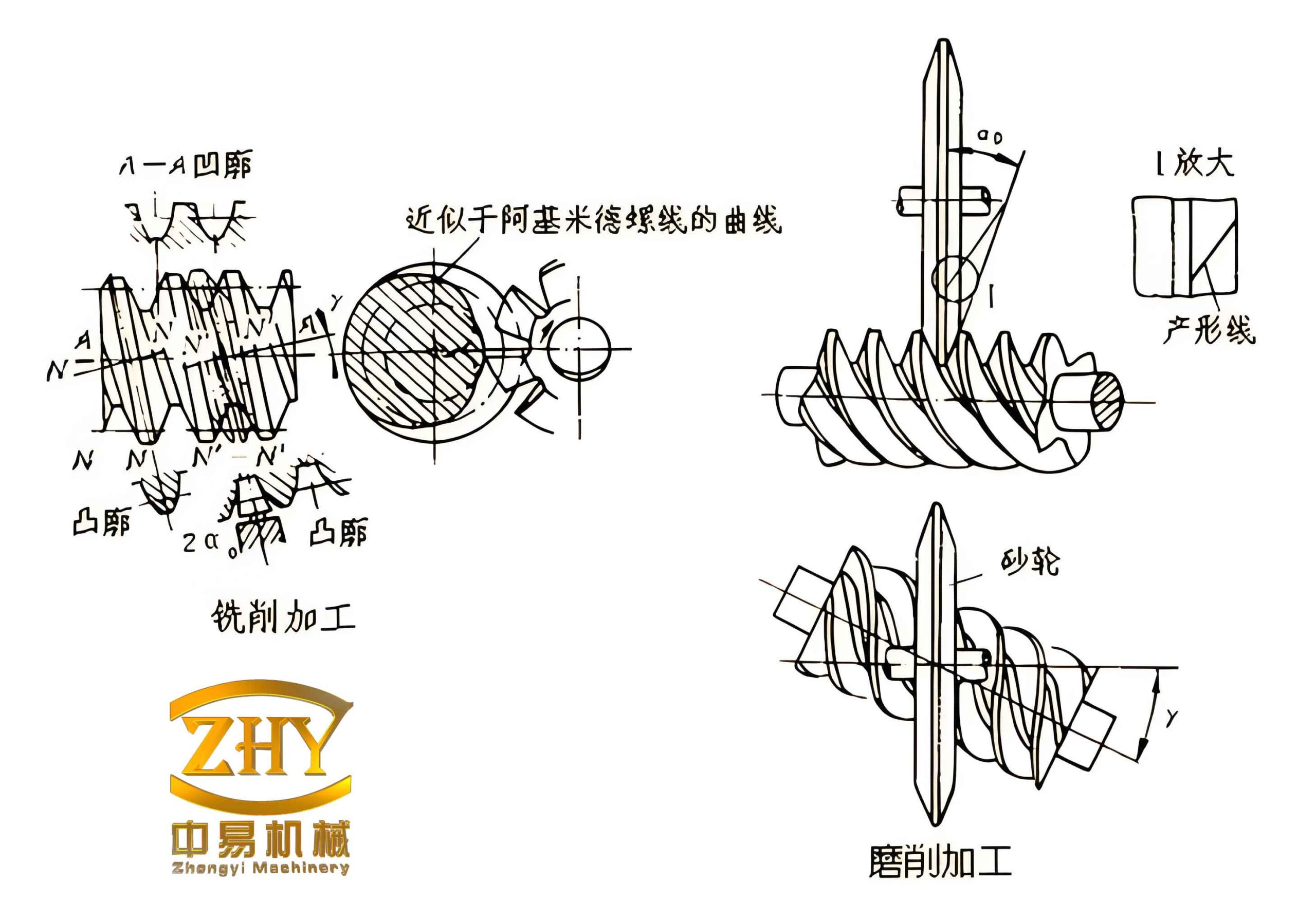
Worm gear drives are widely used in mechanical transmission systems due to their high reduction ratios, smooth operation, and self-locking capability. The three-dimensional modeling of worm gears is essential for modern design and analysis workflows. However, the complex helical tooth surfaces, which must conform to precise kinematic and geometric relationships, pose significant difficulties when using conventional CAD operations. The method presented here simulates the actual manufacturing process of worm gears. For cylindrical worm gears, the tooth surface is typically generated by a straight-edged cutting tool mounted on a lathe. The position and orientation of the tool determine the resulting tooth profile in cross-section. Common types include ZA (Archimedean), ZI (involute), and ZN (normal straight-sided) worms. Each requires a distinct tool geometry and assembly procedure.
Utilizing the ActiveX Automation Interface of MDT 6.0, I developed Visual Basic programs to automate the creation of worm and worm gear models. The core idea is to define a 2D tool profile as a sketch, then sweep that sketch along a 3D helical path to cut the tooth space from a cylindrical blank. For multi-start worms, the resulting tooth slot feature is arrayed around the axis. This technique ensures high precision of the axial tooth profile, as it relies on the accurate helical path rather than approximated lofting between cross-sections.
Methodology for Worm Modeling
The worm modeling process replicates the turning operation used in manufacturing. The cutting tool is represented as a closed polyline in a plane that contains the worm axis (for ZA worms) or offset by the base circle radius (for ZI worms). The tool profile coordinates are computed based on standard worm gear parameters. Table 1 summarizes the key parameters and their notations.
| Symbol | Description |
|---|---|
| $m$ | Modulus |
| $q$ | Diameter coefficient of the worm |
| $Z_1$ | Number of worm threads (starts) |
| $Z_2$ | Number of worm wheel teeth |
| $\alpha$ | Pressure angle |
| $h_a^*$ | Addendum coefficient |
| $c^*$ | Clearance coefficient |
| $L$ | Length of the worm blank |
| $Pitch$ | Lead of the helical path ($\pi m Z_1$) |
For an Archimedean worm (ZA), the cutting tool lies in the axial plane. The tool profile consists of straight lines and a circular arc at the root. The coordinates of the six defining points are given by the following equations:
$$X_1 = 0,\quad Y_1 = m q – (h_a^* + c^*) m$$
$$X_2 = c^* m,\quad Y_2 = Y_1$$
$$X_3 = \frac{\pi m}{4} – h_a^* m \tan\alpha,\quad Y_3 = c^* m + Y_1$$
$$X_4 = \frac{\pi m}{4} + h_a^* m \tan\alpha,\quad Y_4 = (2h_a^* + c^*) m + Y_1$$
$$X_5 = X_4,\quad Y_5 = 1.5 Y_1$$
$$X_6 = 0,\quad Y_6 = Y_5$$
The arc between points 1 and 2 has a specified bulge value to create the root fillet. The remaining segments are straight lines. In the Visual Basic code, these points are stored in a two-dimensional array and used to create a lightweight polyline via the AddLightWeightPolyline method. The polyline is then converted into a sketch entity using AddSketch. The key VB statements are:
Set curves(0) = MDTapp.ActiveDocument.ModelSpace.AddLightWeightPolyline(points)
skdescrip.Selections = curves
Set sketch = part.AddSketch(skdescrip)
To set the bulge for the arc, the method curves(0).SetBulge 1, 0.2 is used.
The worm blank is created as a cylinder with diameter equal to the worm outer diameter and length L. A helical path is defined using the mcHelicalPath sketch descriptor. The lead is calculated as $Pitch = \pi m Z_1$, and the number of revolutions as $Revolutions = L / Pitch$. The tool sketch is then swept along the helical path using a cut operation (mcCut). For a multi-start worm, the resulting slot is polar-arrayed around the axis with $Z_1$ copies. The essential VB calls are:
Set extrude = util.CreateFeatureDescriptor(mcExtrusion)
Set helical = util.CreateSketchDescriptor(mcHelicalPath)
Set helicalSketch = part.AddSketch(helical)
Set sweepDesc = util.CreateFeatureDescriptor(mcSweep)
sweepDesc.Profile = sketch
sweepDesc.CombineType = mcCut
sweepDesc.Path = helicalSketch
Set desc = util.CreateFeatureDescriptor(mcPolarArray)
For involute worm (ZI), the tool is composed of two separate cutting edges, each representing one side of the tooth. They are positioned above and below the worm axis by the base circle radius $r_b = (m q / 2) \cos\alpha$. The coordinates of the left and right tool halves are derived similarly, but only one half of the symmetric profile is used per tool.
Methodology for Worm Wheel Modeling
Modeling the worm wheel (worm gear) follows a similar principle: a cutting tool profile is swept along a helical path to cut the tooth spaces from a cylindrical blank. However, the tool profile is now defined in the transverse plane (end face) of the worm wheel. Figure 2(a) in the original work illustrates the tool shape. The tooth space boundary is composed of a straight line at the root, a circular arc, an involute curve, and another straight line near the tip. The coordinates of the seven defining points are calculated from the gear geometry.
Table 2 lists the formulae for the worm wheel tooth profile.
| Point | $X$ coordinate | $Y$ coordinate |
|---|---|---|
| 1 | $0$ | $R_f$ |
| 2 | $R_f \sin(\theta_3/3)$ | $R_f \cos(\theta_3/3)$ |
| 3 | $R_b \sin\theta_3$ | $R_b \cos\theta_3$ |
| 4 | $R \sin(\theta_3 + \tan\alpha – \alpha)$ | $R \cos(\theta_3 + \tan\alpha – \alpha)$ |
| 5 | $R_a \sin(\theta_3 + \tan\alpha – \alpha)$ | $R_a \cos(\theta_3 + \tan(A\cos(R_b/R_a)) – \arccos(R_b/R_a))$ |
| 6 | $X_5$ | $Y_5 + 2.25 m$ |
| 7 | $0$ | $Y_6$ |
Where:
$$R = \frac{m Z_2}{2},\quad R_a = R + h_a^* m,\quad R_f = R – (h_a^* + c^*) m,\quad R_b = R \cos\alpha$$
$$S_b = \cos\alpha \left( \frac{\pi m}{2} + m Z_2 (\tan\alpha – \alpha) \right)$$
$$\theta_3 = \frac{\pi m \cos\alpha – S_b}{2 S_b}$$
The profile is constructed using three segments: points 1-2-3 form a polyline with a bulge at point 2; points 3-4-5 form a spline representing the involute; points 5-6-7 form another polyline. The entire tool is mirrored about the Y-axis to create the symmetric tooth space. The sketch is created by first drawing the right half, then using the Mirror method to generate the left half.
The worm wheel blank is a cylinder with diameter equal to the outer diameter $2R_a$ and face width $B$. The helical path for the sweep is defined on the surface of this cylinder. Its lead is given by:
$$Pitch = 2\pi R_a \tan\left(\frac{\pi}{2} – \beta\right)$$
where $\beta$ is the helix angle of the worm wheel (typically equal to the lead angle of the worm). The number of revolutions along the path is $Revolutions = B / Pitch$. After creating the cut feature using the sweep operation, the resulting tooth slot is polar-arrayed $Z_2$ times around the blank axis.
The accuracy of the worm gear model depends on the number of fitting points used in the spline definition for the involute curve. The more points taken from the involute equation, the smoother and more precise the tooth profile becomes. Because the sweep operation follows a true helical trajectory, the axial profile is exact, avoiding the approximations inherent in multi-section lofting methods.
Practical Example and Results
To demonstrate the method, I modeled a double-start Archimedean worm drive with the following parameters: $m = 5$, $q = 10$, $Z_1 = 2$, $Z_2 = 31$, $\alpha = 20^\circ$, $h_a^* = 1$, $c^* = 0.2$. The worm blank length was set to 100 mm. The resulting three-dimensional models exhibited smooth, continuous tooth surfaces as shown in the figure below.
The surface quality was verified by examining the intersection curves with axial planes. No visible faceting or discontinuities were observed, confirming the effectiveness of the helical sweep technique. The same approach can be extended to other worm gear types (e.g., ZI, ZN) by modifying the tool geometry and its position relative to the worm axis.
Discussion and Comparison of Modeling Approaches
Several alternative methods exist for worm gear modeling in CAD systems. A common approach is to create a series of cross-sectional profiles along the axis and then loft (or blend) them together. However, the accuracy of lofted surfaces is limited by the number of sections; a large number is required to achieve smoothness, which increases computational cost and file size. The helical sweep method presented here uses a single path and a single profile, producing an analytically exact helical surface. The only approximation comes from the spline representation of the involute curve, which can be controlled by increasing the number of fit points. Table 3 summarizes a comparison of key attributes.
| Aspect | Helical sweep (this work) | Multi-section lofting |
|---|---|---|
| Accuracy of axial profile | Exact | Approximate (depends on section count) |
| Surface continuity | G1 continuous (smooth) | Can be G1 if sections are dense |
| Computational efficiency | Moderate | Higher for many sections |
| Ease of parameterization | Direct formula-based | Requires iterative coordinate calculation |
| Applicability to various worm types | Easy: change tool profile | Easy in principle |
The ActiveX Automation approach allows full parameterization of the worm gear design. By modifying input parameters (modulus, number of teeth, pressure angle, etc.) in the Visual Basic program, a new model can be generated automatically within seconds. This makes the method ideal for design optimization studies and family part generation.
Implementation Details in MDT
The secondary development environment requires MDT 6.0 or later, with the ActiveX type library references added to the Visual Basic project. The following steps outline the program flow:
- Initialize the MDT application and obtain the active document.
- Prompt the user or read parameter values from an input file.
- Create the worm or worm wheel blank as a cylinder using
AddCircleand extrusion. - Compute the tool profile coordinates and create the sketch.
- Define the helical path using the
mcHelicalPathsketch descriptor. Set the diameter, lead, and number of turns. - Perform the sweep cut operation.
- For multi-start worms or multiple gear teeth, apply a polar array feature.
- Optionally, add chamfers, fillets, and center bores.
- Save the model or export for further analysis.
The code relies heavily on the MDT API’s feature descriptors. Understanding the object model is essential. The CreateFeatureDescriptor method creates descriptors for extrusion, sweep, polar array, etc. The CombineType property specifies whether the sweep adds material or cuts. The Profile and Path properties accept sketch objects.
Mathematical Foundation for the Involute Profile
The involute curve used in the worm wheel tooth profile is defined parametrically. For a base circle radius $R_b$, the involute coordinates are:
$$x = R_b (\cos\theta + \theta \sin\theta)$$
$$y = R_b (\sin\theta – \theta \cos\theta)$$
where $\theta$ is the roll angle. In the worm wheel end-face, the involute starts at the base circle and ends at the addendum circle. The angle $\theta_3$ in Table 2 corresponds to the roll angle at the base circle where the involute begins. The point 4 and 5 coordinates were approximated using the tangent and arccos functions; a more rigorous implementation would directly evaluate the involute equation at multiple $\theta$ values and fit a spline through those points. The number of interpolation points can be set by the user to balance accuracy and performance. In the practical example, 20 points were used, which produced a visually perfect involute.
Advantages of the Presented Method
- High geometric accuracy: The helical sweep ensures that every point on the tooth surface lies on the true helix, fulfilling the fundamental law of gearing.
- Full automation: A single execution of the VB program generates the complete worm gear pair, eliminating manual modeling errors.
- Flexibility: The method supports multiple worm types (ZA, ZI, ZN) and various gear parameters. Only the tool profile calculation routine needs to be changed.
- Integration with analysis: The resulting solid models can be directly imported into finite element or computational fluid dynamics software for further study.
- Educational value: The combination of Visual Basic programming and MDT provides a hands-on understanding of gear geometry and CAD automation.
Conclusion
I have presented a practical and efficient approach for creating three-dimensional solid models of worm gears using MDT secondary development. By exploiting the ActiveX Automation Interface and the built-in helical sweep feature, the method produces accurate tooth surfaces that match the theoretical geometry. The Visual Basic code is straightforward to write and modify, making it accessible to engineers and researchers with basic programming skills. The resulting worm gear models are suitable for a wide range of applications, including design verification, kinematic simulation, stress analysis, and manufacturing process planning. Future work may extend this technique to other types of gears, such as bevel gears and hypoid gears, and integrate the model generation with optimization algorithms for automated gear design.