
In this article, I delve into the intricate process of digitally modeling hyperboloid gears and analyzing their time-varying meshing characteristics under various operational conditions. Hyperboloid gears, also known as hypoid gears, are crucial components in automotive, aerospace, and industrial machinery due to their high load-carrying capacity, compact design, and ability to handle large transmission ratios. The focus here is on gears manufactured using the HFT (Hypoid Formate) method, which involves complex kinematic relationships in machine tool movements. My approach involves simulating the tool trajectory through homogeneous coordinate transformations, deriving tooth surface equations based on surface formation theory and conjugate meshing principles, and establishing a comprehensive mathematical model for the gear pair. I then employ numerical algorithms to solve the meshing equations and perform tooth contact analysis (TCA) to obtain static transmission error and contact patterns. Subsequently, I collect discrete point cloud coordinates for the gear and pinion surfaces to create three-dimensional models, and using finite element analysis (FEA) with ABAQUS software, I investigate the time-varying meshing features under different loads. The results highlight how variations in load significantly impact dynamic meshing forces, transmission error, and meshing stiffness, with curves exhibiting asymmetric characteristics as load increases. This analysis provides a foundation for understanding the transmission behavior and dynamic performance of hyperboloid gears.
Hyperboloid gears are widely used in power transmission systems where non-parallel, intersecting shafts are involved. Their unique geometry allows for offset axes, making them ideal for applications like vehicle differentials. However, the complex tooth geometry poses challenges in accurate modeling and analysis. In my work, I address this by starting with the simulation of the manufacturing process on a cradle-type machine tool. The HFT method for hyperboloid gears involves generating the pinion with a cutter head that has tool tilt and swivel motions, while the gear is formed using a two-sided milling process. To replicate this digitally, I define multiple coordinate systems representing the machine tool components, such as the cutter head, cradle, and workpiece. The kinematic relationships between these systems are expressed using homogeneous transformation matrices, which allow for precise simulation of the tool path.
The fundamental step in modeling hyperboloid gears is to derive the equations for the tooth surfaces and root fillets. For the gear (larger wheel), which is processed via the formate method, I consider a dual-sided cutter head. In the cutter coordinate system \( S_{t2} \), the radial vector \( \mathbf{r}_g \) for a point on the cutting edge is given by:
$$ \mathbf{r}_g = \begin{bmatrix} (r_G – u_g \sin \alpha_2) \cos \theta_g \\ (r_G – u_g \sin \alpha_2) \sin \theta_g \\ -u_g \cos \alpha_2 \\ 1 \end{bmatrix} $$
where \( r_G \) is the cutter tip radius, \( u_g \) is the cutting edge length parameter, \( \theta_g \) is the rotation angle of the cutter, and \( \alpha_2 \) is the tool pressure angle. The unit normal vector \( \mathbf{n}_g \) is derived from the cross product of partial derivatives:
$$ \mathbf{n}_g = \frac{\mathbf{N}_g}{|\mathbf{N}_g|} = \begin{bmatrix} -\cos \alpha_2 \cos \theta_g \\ -\cos \alpha_2 \sin \theta_g \\ \sin \alpha_2 \end{bmatrix} $$
To transform these vectors into the gear coordinate system \( S_2 \), I apply a series of homogeneous transformations that account for machine settings like radial distance \( S_r \), angular position \( q \), axial offset \( X \), vertical offset \( E \), and machine root angle \( \delta_M \). The transformation matrix \( \mathbf{M}_{gs2} \) is constructed as:
$$ \mathbf{M}_{gs2} = \mathbf{T}_1 \cdot \mathbf{T}_2 \cdot \mathbf{T}_3 \cdot \mathbf{T}_4 $$
where each \( \mathbf{T} \) matrix represents a translation or rotation based on machine parameters. The resulting radial vector in \( S_2 \) is:
$$ \mathbf{r}_2 = \mathbf{M}_{gs2} \mathbf{r}_g = [x_2, y_2, z_2, 1]^T $$
and the unit normal vector is:
$$ \mathbf{n}_2 = \mathbf{L}_{gs2} \mathbf{n}_g $$
with \( \mathbf{L}_{gs2} \) being the 3×3 rotational submatrix of \( \mathbf{M}_{gs2} \). To obtain discrete points on the gear tooth surface, I mesh the surface in the axial cross-section, solving for parameters \( u_g \) and \( \theta_g \) that satisfy the coordinate constraints. A similar process is applied for the concave side by adjusting the tool pressure angle and tip radius.
For the root transition surface of the gear, which accounts for the cutter tip fillet, I modify the radial vector to include the fillet radius \( r_{gf} \). The equation becomes:
$$ \mathbf{r}’_g = \begin{bmatrix} (r_G – u_{g0} \sin \alpha_2 \pm r_{gf} \cos \alpha_2 \mp r_{gf} \sin \gamma_g) \cos \theta_g \\ (r_G – u_{g0} \sin \alpha_2 \pm r_{gf} \cos \alpha_2 \mp r_{gf} \sin \gamma_g) \sin \theta_g \\ -u_{g0} \cos \alpha_2 \mp r_{gf} \sin \alpha_2 + r_{gf} \cos \gamma_g \\ 1 \end{bmatrix} $$
where \( u_{g0} \) is the parameter at the junction of the main cutting edge and fillet, and \( \gamma_g \) is the fillet angle. Transforming this to \( S_2 \) allows me to generate points for the root fillet surface, ensuring an accurate geometric model that influences stress analysis.
Moving to the pinion (smaller wheel), processed via the HFT method with tool tilt, the modeling is more complex due to additional motions. In the cutter coordinate system \( S_p \), the radial vector for a point on the pinion cutter is:
$$ \mathbf{r}_p = \begin{bmatrix} (r_P + u_p \sin \alpha_1) \cos \theta_p \\ (r_P + u_p \sin \alpha_1) \sin \theta_p \\ -u_p \cos \alpha_1 \\ 1 \end{bmatrix} $$
where \( r_P \) is the pinion cutter tip radius, \( u_p \) and \( \theta_p \) are parameters, and \( \alpha_1 \) is the tool pressure angle. The unit normal vector is:
$$ \mathbf{n}_p = \begin{bmatrix} -\cos \alpha_1 \cos \theta_p \\ -\cos \alpha_1 \sin \theta_p \\ -\sin \alpha_1 \end{bmatrix} $$
The transformation to the pinion coordinate system \( S_1 \) involves multiple steps accounting for tool tilt angle \( i \), tool swivel angle \( j \), radial setting \( S_{r1} \), angular setting \( q_1 \), and others. The composite transformation matrix \( \mathbf{M}_{ps1} \) is:
$$ \mathbf{M}_{ps1} = \mathbf{T}_a \cdot \mathbf{T}_b \cdot \mathbf{T}_c \cdot \mathbf{T}_d \cdot \mathbf{T}_e \cdot \mathbf{T}_f \cdot \mathbf{T}_g $$
This yields the pinion tooth surface vector:
$$ \mathbf{r}_1 = \mathbf{M}_{ps1} \mathbf{r}_p = [x_1, y_1, z_1, 1]^T $$
and unit normal vector:
$$ \mathbf{n}_1 = \mathbf{L}_{ps1} \mathbf{n}_p $$
Since the pinion generation involves a rolling motion between the cradle and workpiece, I introduce a conjugacy condition through the meshing equation:
$$ \mathbf{n}^{c1}_p \cdot \mathbf{v}^{c1}_p = 0 $$
where \( \mathbf{n}^{c1}_p \) is the unit normal in the machine coordinate system, and \( \mathbf{v}^{c1}_p \) is the relative velocity vector. Solving this along with coordinate constraints provides the parameters \( u_p \), \( \theta_p \), and the pinion rotation angle \( \phi_1 \). For the pinion root fillet, a similar approach as the gear is used, incorporating the fillet radius into the cutter geometry.
To summarize the key parameters used in the modeling of hyperboloid gears, I present the following tables that outline the design and machine settings. These parameters are critical for ensuring accurate digital replication of the gear pair.
| Parameter | Pinion (Drive, Left-Hand) | Gear (Driven, Right-Hand) |
|---|---|---|
| Number of Teeth | 10 | 41 |
| Module (mm) | 4.741 | |
| Shaft Angle (°) | 90 | |
| Offset Distance (mm) | -31.8 (Pinion Below Gear) | |
| Face Width (mm) | 33.637 | 28 |
| Outer Cone Distance (mm) | 117.178 | 101.26 |
| Spiral Angle (°) | 49.9833 | 29.0000 |
| Pitch Cone Angle (°) | 15.5293 | 73.7000 |
| Root Cone Angle (°) | 14.1833 | 68.1333 |
| Parameter | Value |
|---|---|
| Cutter Nominal Diameter (inches) | 7.5 |
| Outer Blade Pressure Angle (°) | -24 |
| Inner Blade Pressure Angle (°) | 17 |
| Blade Edge Distance (inches) | 0.09 |
| Tip Fillet Radius (inches) | 0.04 |
| Machine Root Angle (°) | 68.1333 |
| Horizontal Cutter Distance (mm) | 41.11 |
| Vertical Cutter Distance (mm) | 83.66 |
| Axial Workpiece Setting (mm) | -1.36 |
| Parameter | Concave Side (Outer Blade) | Convex Side (Inner Blade) |
|---|---|---|
| Blade Pressure Angle (°) | 14 | -31 |
| Tip Radius (mm) | 92.456 | 97.917 |
| Tip Fillet Radius (inches) | 0.0025 | 0.0025 |
| Machine Root Angle (°) | -4.3 | -4.3167 |
| Radial Cutter Distance (mm) | 89.8950 | 93.5458 |
| Angular Cutter Position (mm) | 87.1750 | 82.0249 |
| Axial Workpiece Setting (mm) | -2.33 | 2.60 |
| Vertical Workpiece Setting (mm) | 29.87 | 32.52 |
| Tool Tilt Angle (°) | 21.2513 | 18.8262 |
| Tool Swivel Angle (°) | -19.6319 | -34.2973 |
| Cutting Ratio (Roll Rate) | 3.87250 | 4.03515 |
After deriving the tooth surface equations, I discretize the surfaces into point clouds. For both the gear and pinion of the hyperboloid gears, I use a grid of 40 points along the tooth length and 20 points along the tooth height for the main surfaces, and 10 points along the height for the root fillets. This ensures high accuracy in the subsequent 3D model reconstruction. The point clouds are then imported into CAD software to generate spline surfaces, which are combined with solid gear blanks to create the final three-dimensional models through Boolean operations. The resulting digital models of the hyperboloid gears are essential for further analysis, as they capture the complex geometry that influences meshing behavior.
With the digital models in place, I proceed to tooth contact analysis (TCA) to evaluate the meshing characteristics of the hyperboloid gears. For unloaded TCA, I define a common meshing coordinate system \( S_H \) where the gear and pinion surfaces are brought into engagement. The radial vectors and unit normal vectors in \( S_H \) are expressed as functions of the rotation angles \( \phi_{h1} \) for the pinion and \( \phi_{h2} \) for the gear. The contact conditions require that at any instant, the position vectors and unit normals of both surfaces match:
$$ \mathbf{r}^H_1 = \mathbf{r}^H_2, \quad \mathbf{n}^H_1 = \mathbf{n}^H_2 $$
This leads to a system of equations with parameters like \( u_g, \theta_g, u_p, \theta_p, \phi_1, \phi_{h1}, \phi_{h2} \). By fixing \( \phi_{h1} \) as an input and solving iteratively, I obtain the contact points across the tooth surfaces. The static transmission error (STE) is calculated as:
$$ \delta(\phi_{h1}) = (\phi_{h2} – \phi^0_{h2}) – \frac{z_1}{z_2} (\phi_{h1} – \phi^0_{h1}) $$
where \( z_1 \) and \( z_2 \) are the numbers of teeth, and \( \phi^0_{h1}, \phi^0_{h2} \) are initial angles. The contact pattern, which shows the area of contact on the tooth surface under no load, is derived from the instantaneous contact ellipses computed at each point. For the hyperboloid gears in this study, the unloaded contact pattern is centered on the tooth surface, indicating proper alignment based on the machine settings.
To analyze the hyperboloid gears under load, I transition to loaded tooth contact analysis (LTCA) using finite element methods. The 3D models are meshed in Hypermesh software, with careful attention to element size to balance accuracy and computational efficiency. I model the pinion with all teeth and the gear with 18 teeth to capture multi-tooth engagement effects. The mesh is then imported into ABAQUS for static structural analysis. The material properties are set for steel, with an elastic modulus of 209 GPa, density of 7850 kg/m³, and Poisson’s ratio of 0.3. The contact interaction between the hyperboloid gears is defined as “hard” contact with a friction coefficient of 0.1, and the analysis uses C3D8R elements (8-node linear brick, reduced integration). I simulate various operating conditions, with the pinion rotating at 200 RPM and applied torques on the gear ranging from 100 N·m to 6000 N·m, to observe how load affects meshing behavior.
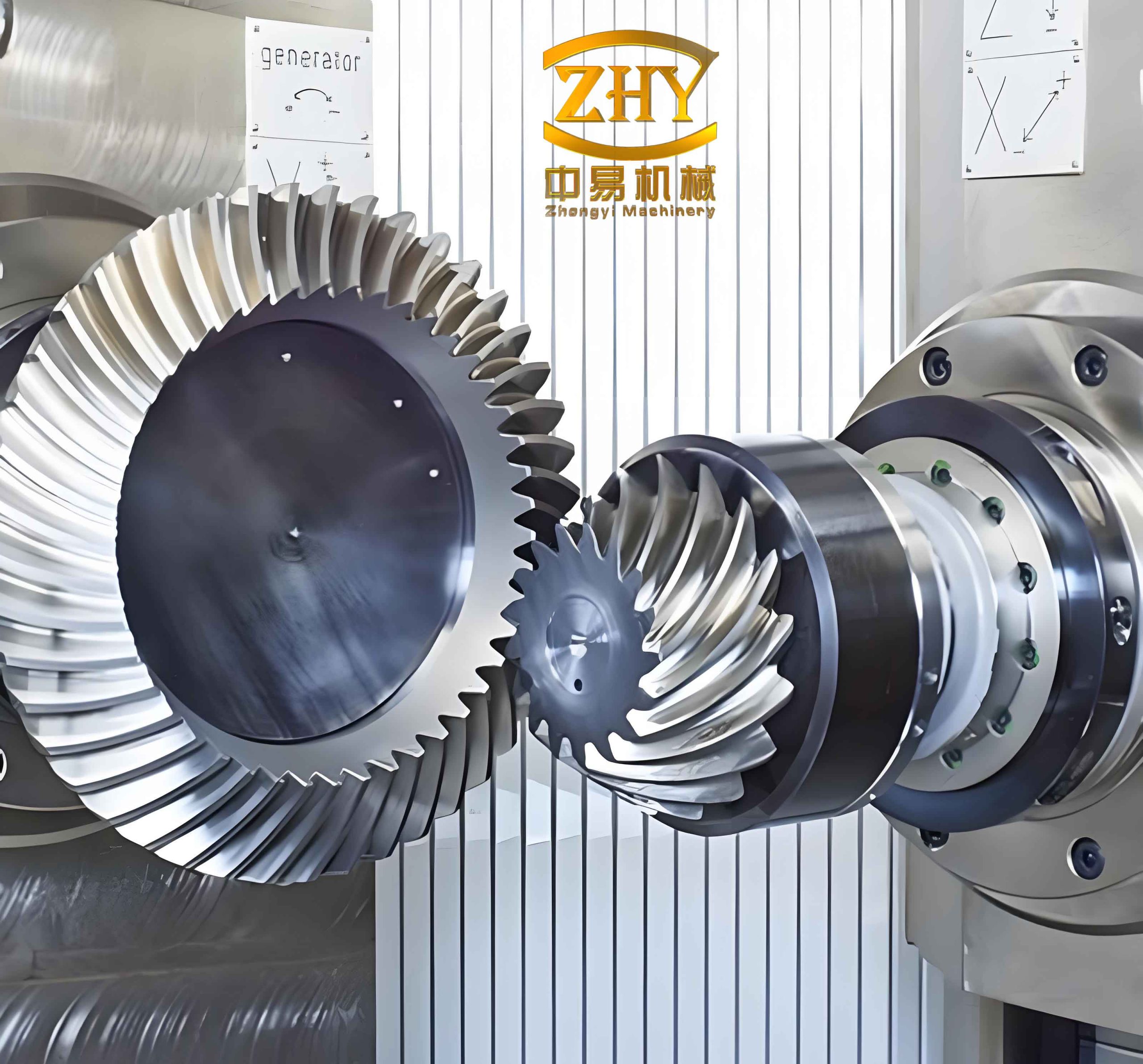
The FEA results provide insights into the time-varying meshing characteristics of the hyperboloid gears. I extract data on dynamic meshing forces, transmission error, meshing stiffness, and actual contact ratio over a mesh cycle. The dynamic meshing force fluctuates with the meshing frequency, and its amplitude increases significantly with load. For instance, at low loads (e.g., 100 N·m), the force variations are minimal, but at high loads (e.g., 6000 N·m), the peaks become pronounced, indicating higher stress concentrations. This is critical for durability assessments of hyperboloid gears in heavy-duty applications.
The transmission error under load shows a similar trend. The unloaded STE curve is relatively smooth, but as load increases, the error fluctuates more intensely. Interestingly, the amplitude of transmission error variation first increases and then decreases with load, suggesting an optimal load range where the contact pattern aligns well with the designed tooth surface. The asymmetry in the transmission error curve becomes evident at higher loads, likely due to shifts in the contact region toward the toe or heel of the tooth. This asymmetry can impact noise and vibration in hyperboloid gear systems.
Meshing stiffness is another key parameter derived from the FEA. I calculate it as the ratio of the meshing force to the elastic deformation of the teeth in the direction of the meshing line. The stiffness varies cyclically during engagement, reflecting the changing number of tooth pairs in contact and the tooth geometry. At low loads, the stiffness curve is nearly symmetric, but with increasing load, the peak stiffness shifts earlier in the mesh cycle. This shift occurs because the contact area moves toward the larger end of the tooth, where the tooth thickness is greater, reducing bending and shear deformations. The stiffness curve thus becomes asymmetric, with a steeper rise and a more gradual decline. This behavior influences the dynamic response of hyperboloid gears, potentially affecting resonance frequencies and stability.
The actual contact ratio, which indicates the average number of tooth pairs in contact during meshing, also varies with load. At light loads, the contact ratio is lower, as only a small portion of the tooth surface is engaged. As load increases, the contact area expands, leading to a higher contact ratio. This increase is rapid initially but plateaus at higher loads, suggesting that beyond a certain point, additional load does not significantly increase the number of contacting teeth. This has implications for load distribution among teeth in hyperboloid gears, especially in applications with fluctuating torques.
To quantify these observations, I present the following table summarizing the time-varying meshing parameters for different load cases. This table encapsulates how hyperboloid gears respond to varying operational conditions, highlighting the sensitivity of meshing characteristics to load changes.
| Load Torque (N·m) | Dynamic Meshing Force Amplitude (N) | Transmission Error Fluctuation (arcsec) | Peak Meshing Stiffness (N/μm) | Actual Contact Ratio |
|---|---|---|---|---|
| 100 | ~500 | ~5 | ~50 | 1.2 |
| 1000 | ~2000 | ~15 | ~180 | 1.8 |
| 3000 | ~6000 | ~25 | ~350 | 2.1 |
| 6000 | ~12000 | ~20 | ~500 | 2.3 |
The contact patterns on the gear tooth surface evolve with load. At low loads, the pattern is concentrated in the central region, but as load increases, it extends toward both the toe and heel, eventually covering almost the entire tooth surface. This expansion improves load distribution but can also lead to edge contacts if not controlled. The starting point of contact shifts toward the larger end of the tooth under higher loads, which aligns with the stiffness behavior observed. These patterns are crucial for optimizing the tooth surface modifications in hyperboloid gears to ensure even wear and reduced stress concentrations.
In conclusion, my digital modeling and analysis of hyperboloid gears reveal that load variations profoundly influence their time-varying meshing characteristics. The methodologies I employed, from kinematic simulations of the manufacturing process to finite element analysis, provide a comprehensive framework for understanding and predicting the behavior of hyperboloid gears in real-world applications. The asymmetric trends in transmission error and meshing stiffness under high loads underscore the need for careful design and tuning of hyperboloid gear systems to mitigate dynamic issues. Future work could explore the effects of misalignments or thermal conditions on these gears, further enhancing their reliability and performance. Overall, this study contributes to the broader knowledge base for hyperboloid gears, offering insights that can guide engineers in developing more efficient and durable power transmission systems.