
In my work I investigate the dynamic behaviour of a compact drive unit in which a rare-earth permanent magnet synchronous machine is combined with a two-stage geared transmission consisting of a spiral bevel pinion gear pair and a planetary gear train. The motivation is straightforward: bucket elevators and similar continuous conveying machines demand light, low-cost and highly integrated drives, and the combination of a high power density permanent magnet motor with a high torque geared reduction stage is an attractive answer. Yet the same integration that brings efficiency also brings vibration. Electromagnetic excitation inside the machine and meshing excitation inside the gearing act simultaneously on the same load path, and the two are coupled through the rotor shaft and the housing. My objective is therefore to build a dynamic model that treats the mechanical transmission and the electrical machine as one system, to quantify the coupling mechanism, and to validate the predictions against measured vibration data.
Description of the Drive Train
The input of the system is a permanent magnet synchronous motor. Torque is delivered to the small spiral bevel pinion gear, transmitted through the meshing contact to the large bevel gear, and then carried by a connecting shaft to the sun gear of the planetary train. The sun gear drives three planet gears, which react against a fixed ring gear, and the output is taken from the carrier. Every rotating component is treated as a rigid body with elastic supports, and the connections between bodies are represented by massless spring-damper elements. This is the classical lumped-mass formulation, and it is well suited to a system in which the number of bodies is modest but the excitation content is rich.
Because the bevel stage transmits load along an axis that is not parallel to the planetary stage, the bevel pinion gear and its mating wheel require a spatial description. I assign four degrees of freedom to each of them, namely three translations and one rotation about the corresponding shaft axis, giving eight degrees of freedom for the bevel pair. The planetary stage, built entirely from spur gearing, is described with a bending–torsion formulation giving six degrees of freedom per body. The complete generalised coordinate vector therefore contains twenty-seven entries.
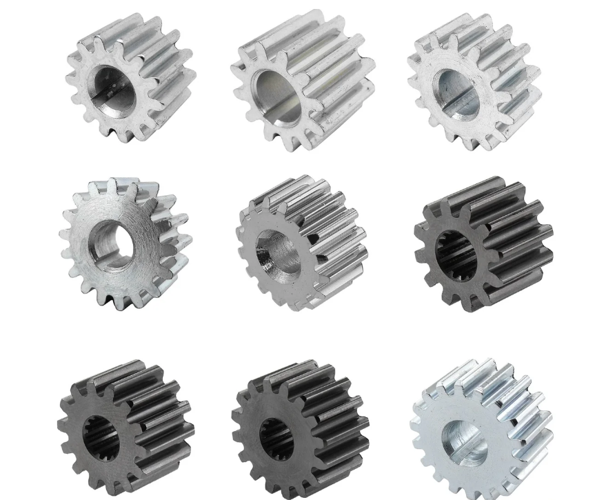
Spiral Bevel Pinion Gear Pair Model
The meshing force acting on the spiral bevel pinion gear tooth flank is written in the standard time-varying form
$$F_n = k_m(t)\,\delta_{12}(t) + c_m\,\dot{\delta}_{12}(t)$$
where $k_m(t)$ is the time-varying mesh stiffness of the bevel pair, $c_m$ is the mesh damping, and $\delta_{12}$ is the relative displacement projected onto the line of action. Projecting the normal load onto the three coordinate axes gives
$$F_x = a_1 F_n, \qquad F_y = a_2 F_n, \qquad F_z = a_3 F_n$$
with the direction coefficients
$$a_1 = \sin\alpha_n\cos\delta_1\cos\beta_1 + \sin\delta_1\sin\alpha_n$$
$$a_2 = \sin\alpha_n\cos\delta_1\sin\beta_1 – \cos\delta_1\sin\alpha_n$$
$$a_3 = \cos\alpha_n\cos\beta_1$$
Here $\alpha_n$ is the normal pressure angle, $\beta_1$ is the mid-face spiral angle of the pinion gear, and $\delta_1$ is its pitch cone angle. The generalised displacement vector of the bevel pair is
$$\mathbf{q}_{pg} = \{x_p,\ y_p,\ z_p,\ \theta_p,\ x_g,\ y_g,\ z_g,\ \theta_g\}^{\mathrm{T}}$$
and the relative displacement along the line of action becomes
$$\delta_{12} = a_1(x_p – x_g) + a_2(y_p – y_g) + a_3(z_p – z_g) + (r_p\theta_p – r_g\theta_g) – e_m(t)$$
where $r_p$ and $r_g$ are the effective base radii at the reference point and $e_m(t)$ is the normal composite meshing error. Applying Newton’s second law to each body yields the eight equations of motion of the bevel stage:
$$\begin{aligned}
m_p\ddot{x}_p + c_{1x}\dot{x}_p + k_{1x}x_p &= -F_x \\
m_p\ddot{y}_p + c_{1y}\dot{y}_p + k_{1y}y_p &= -F_y \\
m_p\ddot{z}_p + c_{1z}\dot{z}_p + k_{1z}z_p &= -F_z \\
I_{xp}\ddot{\theta}_p &= \frac{T_1}{r_p} – \frac{F_n}{r_p} \\
m_g\ddot{x}_g + c_{2x}\dot{x}_g + k_{2x}x_g &= F_x \\
m_g\ddot{y}_g + c_{2y}\dot{y}_g + k_{2y}y_g &= F_y \\
m_g\ddot{z}_g + c_{2z}\dot{z}_g + k_{2z}z_g &= F_z \\
I_{zg}\ddot{\theta}_g &= \frac{T_2}{r_g} – k_u(\theta_g – \theta_s) – \frac{F_n}{r_g}
\end{aligned}$$
In these expressions $m_p$ and $m_g$ are the masses of the pinion gear and wheel, $I_{xp}$ and $I_{zg}$ are the corresponding moments of inertia, $T_1$ and $T_2$ are the input and transfer torques, $k_{ij}$ and $c_{ij}$ are the support stiffness and damping coefficients, and $k_u$ is the torsional stiffness of the connecting shaft.
Planetary Gear Train Model
For the planetary stage I denote the sun by $s$, the carrier by $c$, the ring by $r$ and the planets by $n_1,n_2,n_3$. Each body carries translational coordinates $x_i,y_i$ and a torsional coordinate $\theta_i$, and it is convenient to replace the rotation by the equivalent transverse displacement $u_i = r_i\theta_i$. The sun–planet meshing displacement is
$$\delta_{sn} = \mathbf{V}_{sn}\mathbf{q}_{sn} – e_{sn}(t)$$
with the projection vector
$$\mathbf{V}_{sn} = [\sin\theta_{sn},\ \cos\theta_{sn},\ 1,\ -\sin\alpha,\ -\cos\alpha,\ -1]$$
and the mesh phase angle $\theta_{sn} = \alpha + \phi_{ni}$, where $\phi_{ni}$ is the installation angle of the $i$-th planet. Similarly, the ring–planet meshing displacement is
$$\delta_{rn} = \mathbf{V}_{rn}\mathbf{q}_{rn} – e_{rn}(t)$$
$$\mathbf{V}_{rn} = [\sin\theta_{rn},\ \cos\theta_{rn},\ 1,\ \sin\alpha,\ -\cos\alpha,\ -1]$$
The carrier–planet bearing produces two orthogonal relative displacements
$$\delta_{cnx} = [\cos\theta_{rn},\ \sin\theta_{rn},\ 0,\ -1,\ 0,\ 0]\,\mathbf{q}_{cn}$$
$$\delta_{cny} = [\sin\theta_{rn},\ -\cos\theta_{rn},\ 1,\ 0,\ -1,\ 0]\,\mathbf{q}_{cn}$$
Using the same procedure as before, the governing equations for the four groups of bodies are obtained. For the sun gear,
$$\begin{aligned}
m_s\ddot{x}_s + k_s x_s + \sum_{i=1}^{3} k_{sn}\delta_{sni}\sin\theta_{sni} &= 0 \\
m_s\ddot{y}_s + k_s y_s + \sum_{i=1}^{3} k_{sn}\delta_{sni}\cos\theta_{sni} &= 0 \\
\frac{I_s}{r_s^2}\ddot{u}_s + k_{su}u_s + \sum_{i=1}^{3} k_{sn}\delta_{sni} &= \frac{T_p}{r_s}
\end{aligned}$$
for each planet,
$$\begin{aligned}
m_n\ddot{x}_{ni} – k_{cn}\delta_{cnxi} – k_{sn}\delta_{sni}\sin\alpha + k_{rn}\delta_{rni}\sin\alpha &= 0 \\
m_n\ddot{y}_{ni} – k_{cn}\delta_{cnyi} + k_{sn}\delta_{sni}\cos\alpha – k_{rn}\delta_{rni}\cos\alpha &= 0 \\
\frac{I_n}{r_n^2}\ddot{u}_{ni} – k_{rn}\delta_{rni} + k_{sn}\delta_{sni} &= 0
\end{aligned}$$
for the ring,
$$\begin{aligned}
m_r\ddot{x}_r + k_r x_r + \sum_{i=1}^{3} k_{rn}\delta_{rni}\sin\theta_{rni} &= 0 \\
m_r\ddot{y}_r + k_r y_r – \sum_{i=1}^{3} k_{rn}\delta_{rni}\cos\theta_{rni} &= 0 \\
\frac{I_r}{r_r^2}\ddot{u}_r + k_{ru}u_r + \sum_{i=1}^{3} k_{rn}\delta_{rni} &= 0
\end{aligned}$$
and for the carrier,
$$\begin{aligned}
m_c\ddot{x}_c + k_c x_c + \sum_{i=1}^{3}\left(k_{cn}\delta_{cnxi}\cos\theta_{ni} + k_{cn}\delta_{cnyi}\sin\theta_{ni}\right) &= 0 \\
m_c\ddot{y}_c + k_c y_c + \sum_{i=1}^{3}\left(k_{cn}\delta_{cnxi}\sin\theta_{ni} – k_{cn}\delta_{cnyi}\cos\theta_{ni}\right) &= 0 \\
\frac{I_c}{r_c^2}\ddot{u}_c + k_{cu}u_c + \sum_{i=1}^{3} k_{cn}\delta_{cnyi} &= \frac{T_g}{r_c}
\end{aligned}$$
Combining the bevel equations with the planetary equations gives the assembled system
$$\mathbf{M}\ddot{\mathbf{q}} + \mathbf{C}\dot{\mathbf{q}} + \mathbf{K}\mathbf{q} = \mathbf{F}(t) + \mathbf{e}(t)$$
where $\mathbf{M}$, $\mathbf{C}$ and $\mathbf{K}$ are the global mass, damping and stiffness matrices, $\mathbf{F}$ is the external load vector and $\mathbf{e}$ collects the internal excitations, principally the composite meshing errors.
Numerical Solution Strategy
I solve the assembled equations with the Newmark implicit integration scheme, which is unconditionally stable for the parameter range $\alpha \geq 0.25(0.5+\beta)^2$ and $\beta \geq 0.5$. The recursive relations are
$$\dot{x}_{t+\Delta t} = \dot{x}_t + \Delta t\left[(1-\beta)\ddot{x}_t + \beta\ddot{x}_{t+\Delta t}\right]$$
$$x_{t+\Delta t} = x_t + \Delta t\,\dot{x}_t + \Delta t^2\left[\left(\tfrac{1}{2}-\alpha\right)\ddot{x}_t + \alpha\ddot{x}_{t+\Delta t}\right]$$
Substituting into the equation of motion at time $t+\Delta t$ gives the effective stiffness system
$$\left[\mathbf{K} + A_1\mathbf{M} + A_2\mathbf{C}\right]x_{t+\Delta t} = \mathbf{F}_{t+\Delta t} + \mathbf{M}\left(A_1 x_t + A_4\dot{x}_t + A_5\ddot{x}_t\right) + \mathbf{C}\left(A_2 x_t + A_3\dot{x}_t + A_6\ddot{x}_t\right)$$
with the integration constants
$$A_1 = \frac{1}{\alpha\Delta t^2},\quad A_2 = \frac{\beta}{\alpha\Delta t},\quad A_3 = \frac{1}{\alpha\Delta t},\quad A_4 = \frac{1}{2\alpha}-1,\quad A_5 = \frac{1}{\alpha}-1,\quad A_6 = \frac{\Delta t}{2}\left(\frac{\beta}{\alpha}-2\right)$$
After the displacement increment is obtained, the velocity and acceleration are recovered from the same recursive relations. Once the displacement field is known, the dynamic transmission error of any mesh is evaluated from
$$\mathrm{DTE} = \mathbf{V}\mathbf{q}$$
and the dynamic meshing force follows from
$$F_{ij}(t) = k_{ij}(t)\,\delta_{ij}(t)$$
Baseline Parameters and Characteristic Frequencies
The transmission studied here is rated at 200 kW and 300 r/min at the input, which corresponds to an input torque of 6366.667 N·m. The principal geometric and inertial data are summarised below.
| Parameter | Pinion gear | Bevel wheel | Sun | Planet | Ring | Carrier |
|---|---|---|---|---|---|---|
| Module (mm) | 10.85 | 10.85 | 4.5 | 4.5 | 4.5 | – |
| Number of teeth | 16 | 57 | 23 | 35 | 93 | – |
| Pressure angle (deg) | 20 | 20 | 20 | 20 | 20 | – |
| Helix angle (deg) | 30 | 30 | 0 | 0 | 0 | – |
| Mass (kg) | 2.14 | 118.73 | 7.38 | 5.20 | 36.71 | 242.75 |
| Inertia (kg·m²) | 0.16 | 5.41 | 0.01 | 0.29 | 1.83 | 7.03 |
| Support stiffness (N/m) | 2×10⁹ | 2×10⁹ | 1.18×10⁹ | 5×10⁷ | 7.38×10⁹ | 8.63×10⁸ |
| Torsional stiffness (N·m/rad) | 2.9×10⁹ | 2.9×10⁹ | 3.47×10⁹ | – | 83.40×10⁹ | 3.64×10⁸ |
The corresponding excitation frequencies, obtained from the tooth counts and the shaft speeds, are listed in the next table. They form the reference against which the simulated and measured spectra are interpreted.
| Source | First order (Hz) | Second order (Hz) | Third order (Hz) |
|---|---|---|---|
| Motor rotor | 50 | 100 | 150 |
| Motor stator | 50 | 180 | 360 |
| High-speed shaft | 5 | 10 | 15 |
| Bevel pinion gear mesh | 60 | 120 | 180 |
| Second shaft line | 1.5 | 2.9 | 4.4 |
| Planetary mesh | 25.3 | 50.6 | 75.8 |
Dynamic Response of the Transmission
After the transient has decayed I extract a window of 0.2 s and analyse the steady-state behaviour. The dynamic transmission error of the bevel pinion gear mesh is appreciably larger than that of the planetary meshes because the bevel stage runs at the highest speed, while the planetary meshes carry the largest torque and therefore exhibit the largest force amplitudes. The external and internal planetary meshes show essentially the same waveform shape, differing only by the phase introduced by the planet installation angles.
The dynamic meshing force of the bevel pinion gear pair reaches a maximum of 38.49 kN with a fluctuation band of about 0.12 kN and a mean value near 38.43 kN. In the planetary stage the three external meshes reach peaks of 87.58 kN, 87.48 kN and 87.67 kN respectively, with fluctuation bands between 4.12 kN and 4.51 kN and mean values close to 85.4 kN. The corresponding internal meshes peak at 87.61 kN, 87.60 kN and 87.71 kN with similar fluctuation bands. The small differences between planets originate from the distinct mesh phases rather than from any asymmetry in the geometry.
| Mesh | Peak force (kN) | Fluctuation (kN) | Mean force (kN) |
|---|---|---|---|
| Bevel pinion gear–wheel | 38.49 | 0.12 | 38.43 |
| Sun–planet 1 | 87.58 | 4.12 | 85.47 |
| Sun–planet 2 | 87.48 | 4.42 | 85.32 |
| Sun–planet 3 | 87.67 | 4.51 | 85.55 |
| Ring–planet 1 | 87.61 | 4.24 | 85.46 |
| Ring–planet 2 | 87.60 | 4.40 | 85.54 |
| Ring–planet 3 | 87.71 | 4.49 | 85.54 |
Influence of Input Speed
Holding the transmitted power constant and varying only the input speed produces a clear monotonic trend. Because the torque falls as the speed rises, the meshing force falls with it.
| Input speed (r/min) | Peak external mesh force (kN) |
|---|---|
| 280 | 101.20 |
| 290 | 97.80 |
| 300 | 94.63 |
| 310 | 91.65 |
| 320 | 88.87 |
Influence of Input Power
Holding the speed constant and varying the power produces the opposite trend. Since the torque is proportional to the power at fixed speed, the meshing force grows almost linearly with the power, and for a low-speed heavy-duty drive this dependence dominates the dynamic behaviour.
| Input power (kW) | Peak external mesh force (kN) |
|---|---|
| 180 | 70.54 |
| 190 | 79.58 |
| 200 | 87.58 |
| 210 | 96.81 |
| 220 | 104.94 |
Electromagnetic Finite Element Analysis of the Machine
The electrical machine is a 20-pole, 72-slot surface-mounted permanent magnet synchronous motor rated at 200 kW. I build a two-dimensional finite element model with laminated M470-50A steel for both stator and rotor, copper windings of 1.4 mm conductor diameter, and N38UH permanent magnets. The machine is supplied from a 520 V DC bus through a three-phase inverter in star connection with a phase advance of zero degrees.
| Parameter | Value | Parameter | Value |
|---|---|---|---|
| Poles / slots | 20 / 72 | Slot opening (mm) | 3.5 |
| Stator outer diameter (mm) | 720 | Air gap length (mm) | 1.9 |
| Stator inner diameter (mm) | 510 | Tooth width (mm) | 13.1 |
| Core length (mm) | 640 | d-axis inductance (H) | 0.135 |
| Machine length (mm) | 1100 | q-axis inductance (H) | 0.329 |
| Winding connection | Star | Flux linkage (Wb) | 25.4 |
| Cooling | Water | Phase resistance (Ω) | 111.7 |
| Magnet material | N38UH | Inertia (kg·m²) | 9.5 |
No-Load Back Electromotive Force
The three-phase no-load back electromotive force is symmetric and closely sinusoidal, with a peak amplitude of 257.84 V. The harmonic decomposition is dominated by the first order, and the third-order component is the only other noticeable contribution. All higher orders are small enough to be neglected, which indicates a low harmonic content and a consequently good torque quality.
Electromagnetic Force
The stator magnetomotive force, the rotor magnetomotive force and the air-gap permeance are written respectively as
$$f_A(\theta,t) = \sum_{\nu} f_\nu \cos(\nu\theta \pm \omega t)$$
$$f_R(\theta,t) = \sum_{\mu} f_\mu \cos(\mu\theta – \omega t/p_n)$$
$$\lambda_g(\theta) = \lambda_0\left[1 + \sum_{k=1}^{\infty}\lambda_k\cos(kz\theta)\right]$$
The radial air-gap flux density is the product of the total magnetomotive force and the permeance,
$$B_r(\theta,t) = \left[f_A(\theta,t) + f_R(\theta,t)\right]\lambda_g(\theta)$$
and the radial force density follows from the Maxwell stress tensor,
$$P_r(\theta,t) = \frac{1}{2\mu_0}\left(B_r^2 – B_t^2\right) \approx \frac{1}{2\mu_0}B_r^2$$
The simulated flux density reaches 2.217 T at the outer diameter of the stator lamination and in the rotor yoke. Under no-load conditions the dominant radial force harmonic is the twentieth order with an amplitude of 0.3075 kN, and weaker components appear at the 32nd, 40th and 52nd orders. Under load the corresponding dominant amplitude rises slightly to 0.3086 kN. The tangential force is far weaker throughout: its dominant harmonic is the 140th order with an amplitude of 0.0346 kN at no load and 0.0351 kN under load. Because the radial component exceeds the tangential component by roughly an order of magnitude, the radial force is the controlling excitation for stator vibration, and I concentrate the parametric study on it.
| Condition | Dominant radial order | Radial amplitude (kN) | Dominant tangential order | Tangential amplitude (kN) |
|---|---|---|---|---|
| No load | 20 | 0.3075 | 140 | 0.0346 |
| Rated load | 20 | 0.3086 | 140 | 0.0351 |
Effect of Slot Opening Width on Radial Force
Increasing the slot opening has two consequences that act in the same direction: it strengthens the permeance harmonics and it amplifies the force wave produced by the squared tooth harmonic component. The result is a monotonic growth of the radial force.
| Slot opening (mm) | Peak radial force (kN) |
|---|---|
| 2.5 | 0.7308 |
| 3.0 | 0.7451 |
| 3.5 | 0.7694 |
| 4.0 | 0.7730 |
| 4.5 | 0.8032 |
| 5.0 | 0.8213 |
Effect of Air Gap Length on Radial Force
Enlarging the air gap raises the reluctance and therefore reduces the force, but an excessive gap degrades the power factor. A compromise value must be selected.
| Air gap (mm) | Peak radial force (kN) |
|---|---|
| 1.5 | 0.8626 |
| 1.6 | 0.8333 |
| 1.7 | 0.8130 |
| 1.8 | 0.7847 |
| 1.9 | 0.7694 |
| 2.0 | 0.7610 |
Cogging Torque
The cogging torque is evaluated both from the Maxwell stress integral and from the virtual work principle. In the stress formulation
$$T = \frac{r}{\mu_0}\oint_{S} B_r B_t\,\mathrm{d}S$$
while in the virtual work formulation the torque is the sum of the elemental energy derivatives in the air gap,
$$T_{c} = \sum_{i=1}^{N}\frac{\mathrm{d}W_i}{\mathrm{d}\theta_c}$$
Both methods give almost identical curves, which supports the reliability of the computation. For the reference design the peak cogging torque is 0.1318 N·m, small enough to be acceptable for the application.
| Pole / slot combination | Peak cogging torque (N·m) |
|---|---|
| 20 / 48 | 5.2745 |
| 20 / 60 | 2.2450 |
| 20 / 84 | 0.0890 |
| 20 / 96 | 0.0667 |
At a fixed pole number the cogging torque falls as the slot number rises, but a larger slot number also enlarges the stator core diameter and reduces slot utilisation, so the choice is again a compromise.
| Slot opening (mm) | Peak cogging torque (N·m) |
|---|---|
| 2.5 | 0.2461 |
| 3.0 | 0.2137 |
| 3.5 | 0.1318 |
| 4.0 | 0.1500 |
| 4.5 | 0.1569 |
| 5.0 | 0.1599 |
The cogging torque first decreases and then increases with the slot opening, so an intermediate value is optimal. The selected configuration of 20 poles, 72 slots and a 3.5 mm slot opening satisfies the engineering requirement.
Torque Ripple and Efficiency
Over the constant-torque region up to the rated speed of 300 r/min the output torque remains close to 6600 N·m and the deviation band is narrow, which indicates a modest torque ripple and consequently a low excitation level for the mechanical system. Beyond the base speed the machine enters the field-weakening region and the torque falls. The efficiency rises steeply at low speed and stabilises near 98 percent, which meets the design target.
Electromechanical Coupling Model
The permanent magnet synchronous machine is a strongly coupled nonlinear system, and I adopt the usual assumptions of symmetric windings, a sinusoidal air-gap field produced by the magnets, and negligible hysteresis, eddy-current and saturation effects. In the stationary three-phase frame the voltage and flux linkage equations are
$$\mathbf{u}_s = R_s\mathbf{i}_s + \frac{\mathrm{d}\boldsymbol{\Psi}_s}{\mathrm{d}t}, \qquad \boldsymbol{\Psi}_s = \mathbf{L}_s\mathbf{i}_s + \psi_f\mathbf{F}_s(\theta_e)$$
After the Clarke and Park transformations the machine is described in the rotating frame by the flux linkages
$$\psi_d = L_d i_d + \psi_f, \qquad \psi_q = L_q i_q$$
the voltage equations
$$\begin{aligned}
u_d &= R_s i_d + L_d\frac{\mathrm{d}i_d}{\mathrm{d}t} – \omega_e L_q i_q \\
u_q &= R_s i_q + L_q\frac{\mathrm{d}i_q}{\mathrm{d}t} + \omega_e\left(L_d i_d + \psi_f\right)
\end{aligned}$$
and the electromagnetic torque
$$T_e = \frac{3}{2}p_n\left[i_q\psi_f + (L_d – L_q)i_d i_q\right]$$
The mechanical balance of the rotor, including its elastic connection to the bevel pinion gear shaft, becomes
$$J_m\ddot{\theta}_m = T_e – k_{u1}(\theta_m – \theta_p) – c_{u1}(\dot{\theta}_m – \dot{\theta}_p)$$
so that the shaft torque is transmitted to the bevel pinion gear through the same elastic element, and the pinion then drives the remainder of the transmission as described in the previous sections. Combining these equations with the geared system yields the complete electromechanical formulation
$$J_m\frac{\mathrm{d}\omega_m}{\mathrm{d}t} = T_e – T_L – k_{u1}\left(u_{in} – u_{xp}\right)/r_{in}$$
$$\begin{aligned}
m_p\ddot{x}_p + c_{1x}\dot{x}_p + k_{1x}x_p &= -F_x \\
m_p\ddot{y}_p + c_{1y}\dot{y}_p + k_{1y}y_p &= -F_y \\
m_p\ddot{z}_p + c_{1z}\dot{z}_p + k_{1z}z_p &= -F_z \\
I_{xp}\ddot{u}_{xp} – k_{u1}\left(u_{in} – u_{xp}\right) &= -F_n r_p
\end{aligned}$$
together with the planetary equations listed earlier. The coupling is therefore two-way: the electromagnetic torque drives the gear train, and the dynamic meshing forces react back on the rotor as a fluctuating load torque.
Vector Control and Speed Estimation
I adopt the $i_d = 0$ vector control strategy, under which the electromagnetic torque reduces to
$$T_e = \frac{3}{2}p_n i_q\psi_f$$
The speed loop uses a sliding-mode controller. Defining the state variables
$$x_1 = \omega_r – \omega_m, \qquad x_2 = \dot{x}_1 = -\dot{\omega}_m$$
and the sliding surface
$$s = c x_1 + x_2, \qquad c > 0$$
an exponential reaching law gives the control law
$$u = \frac{1}{D}\left[c x_2 + \varepsilon\,\mathrm{sgn}(s) + q s\right], \qquad D = \frac{3p_n\psi_f}{2J}$$
which after integration yields the q-axis current reference
$$i_q^{*} = \frac{1}{D}\int_0^{t}\left[c x_2 + \varepsilon\,\mathrm{sgn}(s) + q s\right]\mathrm{d}\tau$$
The current loops use conventional proportional-integral regulators with feed-forward decoupling,
$$\begin{aligned}
u_d^{*} &= \left(K_{pd} + \frac{K_{id}}{s}\right)\left(i_d^{*} – i_d\right) – \omega_e L_q i_q \\
u_q^{*} &= \left(K_{pq} + \frac{K_{iq}}{s}\right)\left(i_q^{*} – i_q\right) + \omega_e\left(L_d i_d + \psi_f\right)
\end{aligned}$$
with the gains selected from the desired bandwidth $\alpha$ as
$$K_{pd} = \alpha L_d,\quad K_{id} = \alpha R_s,\quad K_{pq} = \alpha L_q,\quad K_{iq} = \alpha R_s$$
The inverter is a six-switch bridge driven by sinusoidal pulse-width modulation. Because there is no shaft-mounted encoder in the target application, rotor position and speed are reconstructed with a model reference adaptive system. Writing the machine in the current form
$$\frac{\mathrm{d}}{\mathrm{d}t}\mathbf{i}’ = \mathbf{A}’\mathbf{i}’ + \mathbf{B}’\mathbf{u}’$$
and denoting the estimated quantities with a hat, the generalised error $\boldsymbol{\varepsilon} = \mathbf{i}’ – \hat{\mathbf{i}}’$ evolves according to
$$\frac{\mathrm{d}\boldsymbol{\varepsilon}}{\mathrm{d}t} = \mathbf{A}’\boldsymbol{\varepsilon} – \mathbf{W}, \qquad \mathbf{W} = (\omega_e – \hat{\omega}_e)\mathbf{J}\hat{\mathbf{i}}’, \qquad \mathbf{J} = \begin{bmatrix} 0 & -1 \\ 1 & 0 \end{bmatrix}$$
Applying the Popov integral inequality gives the adaptive law
$$\hat{\omega}_e = K_p\left(i_d’\hat{i}_q’ – i_q’\hat{i}_d’\right) + K_i\int_0^{t}\left(i_d’\hat{i}_q’ – i_q’\hat{i}_d’\right)\mathrm{d}\tau$$
which is equivalent to
$$\hat{\omega}_e = K_p\left[i_q\hat{i}_d – i_d\hat{i}_q – \frac{\psi_f}{L_s}\left(i_q – \hat{i}_q\right)\right] + \frac{K_i}{s}\left[i_q\hat{i}_d – i_d\hat{i}_q – \frac{\psi_f}{L_s}\left(i_q – \hat{i}_q\right)\right]$$
and the rotor position follows by integration,
$$\hat{\theta}_e = \int_0^{t}\hat{\omega}_e\,\mathrm{d}\tau$$
This arrangement allows reliable identification of the initial rotor magnet position and of the running speed, which is essential for a smooth and stable start under low-speed, high-torque and overload conditions.
Coupled Simulation Results
The complete electromechanical model is implemented with the mechanical subsystem encapsulated in a dedicated block and the control subsystem comprising coordinate transformation, pulse-width modulation, the adaptive observer, the sliding-mode speed controller and the current regulators.
Steady Load
With a speed reference of 300 r/min and zero external load torque, the machine accelerates from rest and reaches the reference speed after approximately one second, after which it remains steady. The stator phase currents settle to an amplitude near 50 A and are essentially sinusoidal. Comparing the coupled response with the purely mechanical prediction reveals that the dynamic transmission error of the bevel pinion gear mesh has a larger amplitude and a wider fluctuation band once the electrical machine is included, and that the planetary meshes likewise exhibit larger mean values and amplitudes.
Spectral analysis of the sun–planet mesh transmission error shows energy concentrated at the zero order together with discrete peaks at approximately 1.429 Hz, 4.286 Hz, 25 Hz, 50 Hz and 60 Hz. These correspond closely to the first and second shaft orders and to the first and second mesh orders of the gear stages. In addition, the spectrum contains electromechanical sidebands in which the electrical harmonics act as carriers and multiples of the gear mesh frequency act as modulating frequencies, so the spectral content of the coupled system is richer than that of either subsystem alone. The high-frequency content is of small amplitude and therefore of limited consequence for the mechanical structure, whereas the low-frequency electrical torque fluctuations are amplified by the coupling and dominate the mechanical response.
For the bevel pinion gear mesh the coupled peak force is 38.56 kN with a mean near 38.51 kN. The sun–planet 1 mesh reaches 94.40 kN with a mean near 83.51 kN, and the ring–planet 1 mesh reaches 92.92 kN with a mean near 83.25 kN. All values exceed the uncoupled predictions, which confirms that the electrical harmonics, cogging effects and spatial harmonics of the machine intensify the torque ripple and thereby increase the load fluctuation seen by the gearing.
| Mesh | Uncoupled peak (kN) | Coupled peak (kN) | Increase (%) |
|---|---|---|---|
| Bevel pinion gear–wheel | 38.49 | 38.56 | 0.18 |
| Sun–planet 1 | 87.58 | 94.40 | 7.79 |
| Ring–planet 1 | 87.61 | 92.92 | 6.06 |
Fluctuating Load
A slowly varying load produces a meshing force whose trend follows the load waveform closely, with peaks noticeably higher than under steady load. The spectral amplitudes change only slightly, because the current, the speed and the mesh force all vary slowly and no new dominant frequency is generated.
Sudden Load Change
When the load is switched abruptly from zero to 50 N·m for a short interval and then removed, the meshing force changes sharply during the loaded interval and remains comparatively calm when the load is absent. The spectral amplitudes change appreciably because the abrupt transition excites the natural modes of the driveline. In general the stronger the load fluctuation and the faster its rate of change, the larger the resulting meshing force and the greater its influence on the dynamic behaviour of the whole system.
| Load case | Force trend | Spectral amplitude change | Peak relative to steady load |
|---|---|---|---|
| Steady | Constant with ripple | Reference | Reference |
| Fluctuating | Follows load waveform | Small | Higher |
| Sudden | Abrupt steps | Large | Much higher |
Experimental Investigation
To validate the model I assembled a test rig consisting of the drive under investigation, a flexible coupling, a torque transducer and a driving machine. Before testing, the assembly was checked for cleanliness and alignment, and the run-out of the coupling flanges was verified. Loading was applied by a back-to-back arrangement with a 390 kW machine, which allowed both no-load and loaded operation to be examined. Vibration was measured with an accelerometer-based acquisition system, rotational speed was monitored with a dedicated sensor, and all signals were recorded and analysed on a computer.
| Item | Description | Item | Description |
|---|---|---|---|
| Driving machine | 400 frame, 20 pole | Universal coupling | Heavy-duty cardan type |
| Torque transducer | 20000 N·m range | Support base | Rigid fabricated base |
| Data acquisition | Eight-channel recorder | High-speed coupling | Flexible disc type |
| Vibration system | Multi-channel analyser | Speed sensor | Magnetic pickup |
Measurement Points
Four measurement points were selected on the housing where the response is expected to be most pronounced. Point 1 is located at the joint between the motor housing and the gearbox, point 2 on the cover directly above the bevel wheel bearing seat, point 3 on the cover above the ring gear of the planetary stage, and point 4 at the rear of the permanent magnet machine near the backstop.
No-Load Results
During the no-load test, vibration velocity was sampled every five minutes before the rated speed was reached and every fifteen minutes afterwards. The spectra at all four points are dominated by peaks near 25 Hz, 60 Hz and 100 Hz, which correspond to the gear mesh frequencies and their multiples. The vibration at the rear of the machine is governed by the electrical load, while the vibration at the planetary housing is produced mainly by the first planetary mesh order together with the second bevel mesh order. The bevel pinion gear region shows a pronounced electromechanical coupling effect, with contributions from both the electrical excitation and the bevel mesh frequency.
Loaded Results
The loaded tests were carried out at 20, 40, 60, 80 and 100 percent of the rated speed for fifteen minutes each, followed by a staged torque loading sequence. Within the rated torque the vibration was sampled every fifteen minutes, and during the 130 percent overload it was sampled every ten minutes.
| Stage | Input torque (N·m) | Torque level | Output torque (N·m) | Duration (h) |
|---|---|---|---|---|
| 1 | 1592 | 25% rated | 320 | 1 |
| 2 | 3184 | 50% rated | 639 | 1 |
| 3 | 4457 | 70% rated | 895 | 1 |
| 4 | 6367 | 100% rated | 1278.5 | Until thermal equilibrium |
| 5 | 8277 | 130% rated | 1662 | 0.5 |
As the load increases, the dominant spectral peaks remain near 25 Hz, 60 Hz and 100 Hz, confirming that the mesh orders and their multiples govern the response at every load level. A number of low-level disturbance frequencies appear at higher loads, but their contribution to the overall vibration is small. The vibration at the rear bearing of the machine is relatively insensitive to load but strongly dependent on speed, with the fundamental electrical frequency dominating, which supports the conclusion that the machine-end vibration originates from the radial and tangential electromagnetic forces. The behaviour at the other three points is consistent with the no-load observations.
Comparison Between Simulation and Measurement
Vibration velocities at the four bearing locations were computed from the coupled model and compared with the measured no-load spectra. The overall trends agree well, and the dominant peaks in both data sets lie near 25 Hz, 60 Hz and 100 Hz, matching the mesh frequencies and their multiples. The measured spectra contain additional low-level components arising from the test environment, which spread the energy over a wider frequency range but do not alter the dominant structure of the response.
| Measurement point | Measured peak (µm/s) | Simulated peak (µm/s) | Deviation (%) |
|---|---|---|---|
| Point 1 – motor–gearbox joint | 353.89 | 373.20 | 5.46 |
| Point 2 – bevel wheel bearing cover | 514.26 | 533.80 | 3.80 |
| Point 3 – ring gear cover | 240.03 | 263.58 | 9.81 |
| Point 4 – rear of the machine | 340.26 | 360.73 | 6.02 |
The deviations range from 3.80 percent to 9.81 percent with a mean of 6.27 percent, which I consider acceptable for a model of this complexity and which supports the validity of the coupled formulation. The origin of the vibration differs from point to point. At the rear of the machine and at the motor–gearbox joint the excitation is predominantly electromagnetic. At the planetary housing it is the first planetary mesh order combined with the second bevel mesh order. At the bevel pinion gear region both the electrical excitation and the bevel mesh frequency contribute, which is the clearest experimental evidence of the electromechanical coupling described in the simulation.
Concluding Remarks
The work reported here leads to several conclusions that I consider useful for the design of integrated permanent magnet motor and gear drive units.
The lumped-mass formulation with a bending–torsion–axial description of the bevel stage and a bending–torsion description of the planetary stage captures the essential dynamics of the transmission. The dynamic meshing force increases with transmitted power and decreases with input speed, and for a low-speed heavy-duty drive the power dependence is the stronger of the two.
The electromagnetic analysis shows that the radial force dominates the tangential force by roughly an order of magnitude and that its harmonic orders are integer multiples of the pole number. The radial force grows with the slot opening and falls with the air-gap length. The cogging torque falls as the slot number increases at a fixed pole number, and it exhibits a minimum at an intermediate slot opening, so both quantities require a compromise in the design of the machine.
The coupled simulation demonstrates a genuine two-way interaction. The mechanical vibration introduces additional harmonic content into the electromagnetic torque, and the electrical harmonics and cogging effects introduce additional harmonic content into the meshing forces. The result is a spectrum containing sidebands in which the electrical harmonics act as carriers and the mesh frequency multiples act as modulators. Under fluctuating and sudden loads the meshing force tracks the load waveform and reaches peaks substantially higher than under steady load, while under slowly varying load the spectral amplitudes are comparatively insensitive to the load level.
The experimental campaign confirms the model. The measured dominant frequencies at the four housing locations coincide with the predicted mesh orders and their multiples, the measured and simulated peak vibration velocities agree within a mean deviation of about six percent, and the spatial distribution of the vibration sources matches the physical interpretation derived from the coupled model.
Further work should refine the tooth contact analysis of the spiral bevel pinion gear and of the internal planetary meshes, because the contact state varies appreciably from one meshing position to the next and influences the effective stiffness. Additional factors that deserve attention include friction in the shaft and bearing interfaces, rotor eccentricity and the unbalanced magnetic pull it produces, and the combined effect of spatial and temporal harmonics on the coupled response. Extending the parametric study to a wider range of operating conditions would also improve the generality of the conclusions.