
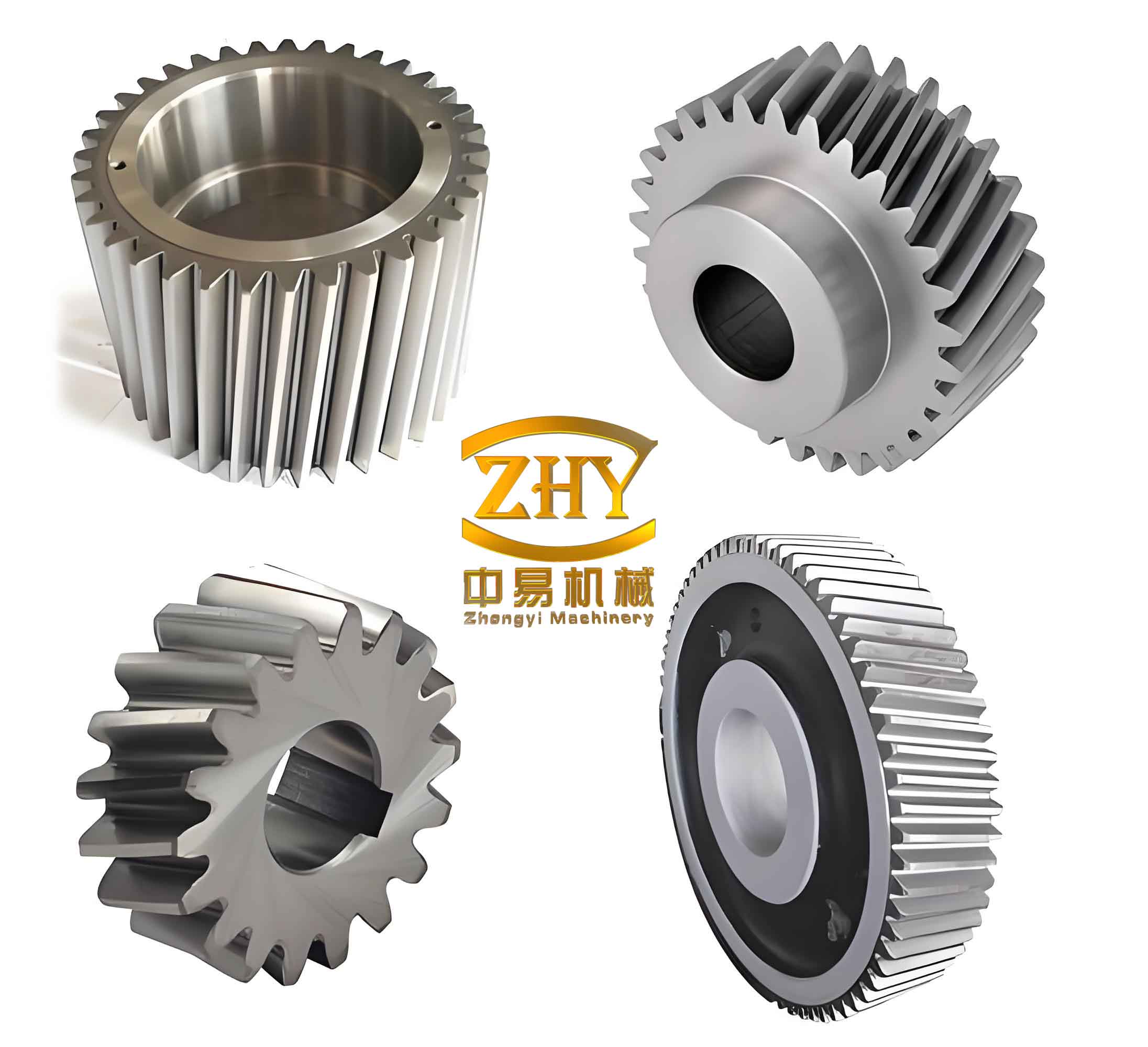
I treat the shifted helical gear transmission system as a coupled mechanical system in which geometric profile shift, time-varying mesh stiffness, dynamic mesh force, dynamic transmission error, and axial vibration acceleration are strongly connected. My objective is to formulate an analytical and dynamic framework that can describe how profile shift changes the behavior of a helical gear pair and how the shift coefficients can be optimized for low dynamic force and low transmission error. The work combines slice theory, energy-based stiffness calculation, an eight-degree-of-freedom dynamic model, experimental validation, and a multi-objective genetic algorithm. The resulting method is intended for practical rail-transit and industrial helical gear systems where reliability, acoustic behavior, and fatigue life are important.
1. Research Context and Technical Logic
Helical gear drives are widely used because they provide smooth meshing, large contact ratio, compact layout, and good load capacity. Compared with spur gears, a helical gear pair has an inclined contact line, so the mesh stiffness is not constant along the face width. The contact line grows, remains full, and then shrinks during one mesh cycle. This behavior makes the time-varying mesh stiffness of a helical gear more complex than that of a spur gear. When profile shift is introduced, the tooth thickness, addendum, dedendum, center distance, and mesh angle all change. These changes alter the contact ratio, the effective contact line, and the stiffness components, which in turn affect the dynamic response.
I divide the problem into four main parts. First, I calculate the time-varying mesh stiffness of a shifted helical gear pair by slicing the gear along the face width and integrating the contributions of all slices. Second, I establish an analytical model for the shifted helical gear and validate it with finite element analysis. Third, I build an eight-degree-of-freedom dynamic model of the shifted helical gear transmission system and verify it experimentally. Fourth, I optimize the profile shift coefficients using a non-dominated sorting genetic algorithm. The overall logic is shown by the following relation:
$$ \text{Profile shift} \rightarrow \text{geometry change} \rightarrow \text{mesh stiffness change} \rightarrow \text{dynamic response change} \rightarrow \text{multi-objective optimization}. $$
Because the helical gear contact line is inclined, the mesh stiffness calculation must account for the instantaneous contact length. I therefore use the slice method as the foundation. Each thin slice is treated as a spur gear slice, and the total stiffness is obtained by summing or integrating the slice stiffnesses. This approach preserves the helical gear characteristics while keeping the calculation efficient.
2. Slice Model and Time-Varying Contact Line of a Helical Gear
For a helical gear, the contact line is not parallel to the axis. It moves across the tooth surface as the gear rotates. At the beginning of engagement, the contact line is short. It then increases until it spans the full face width. After that, it decreases until disengagement. I define the instantaneous contact line length as \(l(\mu)\), where \(\mu\) is the distance from the initial engagement point. The contact line length can be expressed as:
$$ l(\mu)= \begin{cases} \mu \cot\beta_b, & 0 \le \mu \le L_1,\\ L_2, & L_1 \le \mu \le L_1+L_2,\\ (L_1+L_2+L_3-\mu)\cot\beta_b, & L_1+L_2 \le \mu \le L_1+L_2+L_3, \end{cases} $$
where \(\beta_b\) is the base helix angle, \(L_1\), \(L_2\), and \(L_3\) are the lengths of the three contact-line stages, and the total face width is \(B\). The base helix angle is related to the helix angle and the transverse pressure angle by:
$$ \tan\beta_b = \tan\beta \cos\alpha_t. $$
The transverse contact ratio of the helical gear pair is:
$$ \varepsilon_\alpha = \frac{Z_1(\tan\alpha_{at1}-\tan\alpha’)+Z_2(\tan\alpha_{at2}-\tan\alpha’)}{2\pi}, $$
where \(Z_1\) and \(Z_2\) are the tooth numbers of the pinion and gear, \(\alpha_{at1}\) and \(\alpha_{at2}\) are the transverse addendum pressure angles, and \(\alpha’\) is the working transverse pressure angle. The axial contact ratio is:
$$ \varepsilon_\beta = \frac{B\sin\beta}{\pi m_n}, $$
and the total contact ratio is:
$$ \varepsilon = \varepsilon_\alpha + \varepsilon_\beta. $$
For a helical gear pair with \(2<\varepsilon<3\), the mesh cycle contains both two-tooth and three-tooth contact regions. This is important because the comprehensive time-varying mesh stiffness is not simply the sum of single-tooth stiffnesses. The engagement sequence must be considered. I define the mesh period as \(T_m=2\pi/N\), where \(N\) is the number of teeth on the reference gear, and the single-tooth mesh period as \(T_t=\varepsilon T_m\). During one mesh period, the load is shared by two or three tooth pairs, and the comprehensive stiffness is obtained by adding the contributions of all active tooth pairs.
3. Analytical Model for Shifted Helical Gear Mesh Stiffness
Profile shift changes the tooth geometry while preserving the same involute. The addendum and dedendum of the shifted helical gear are:
$$ h_{ai} = (h_a^* + x_{ni} – \Delta y_n)m_n, $$
$$ h_{fi} = (h_a^* + c^* – x_{ni})m_n, $$
where \(h_a^*\) is the addendum coefficient, \(c^*\) is the clearance coefficient, \(x_{ni}\) is the normal profile shift coefficient of gear \(i\), \(\Delta y_n\) is the addendum reduction coefficient, and \(m_n\) is the normal module. The working center distance and the working transverse pressure angle are:
$$ a_i = \frac{(Z_1+Z_2)\cos\alpha_{0t}}{2\cos\alpha_t}m_t, $$
$$ \operatorname{inv}\alpha_t = \operatorname{inv}\alpha_{0t} + \frac{2\tan\alpha_n(x_1+x_2)}{Z_1+Z_2}. $$
The angle between the base circle tooth root and the tooth centerline is:
$$ \alpha_2 = \frac{s}{2r} + \operatorname{inv}\alpha = \frac{\pi}{Z} + \frac{2x\tan\alpha_n}{Z} + \operatorname{inv}\alpha. $$
The initial transverse mesh pressure angles of the pinion and gear are:
$$ \alpha_{p0} = \tan\alpha_{p} – \arccos\left(\frac{r_{bp}}{r_{ap}}\right), $$
$$ \alpha_{g0} = \tan\alpha_{g} – \arccos\left(\frac{r_{bg}}{r_{ag}}\right). $$
After the gear rotates, the instantaneous mesh angle of the \(i\)-th slice is updated by the rotation angle. For the pinion and gear, the angles can be written as:
$$ \alpha_1(i) = \alpha_{p0} + \theta_1(i), $$
$$ \alpha_1′(i) = \alpha_{g0} – \frac{\theta_1(i)}{i}, $$
where \(i=Z_2/Z_1\) is the transmission ratio. These angles determine the position of the load on the tooth profile and therefore affect every stiffness component.
4. Stiffness Components of a Shifted Helical Gear Slice
Using the energy method, I decompose the single-tooth mesh stiffness into five parts: Hertz contact stiffness, bending stiffness, shear stiffness, axial compressive stiffness, and fillet-foundation stiffness. The Hertz contact stiffness of a slice is:
$$ k_h = \frac{\pi E B}{4(1-\nu^2)}, $$
where \(E\) is the elastic modulus, \(\nu\) is the Poisson ratio, and \(B\) is the face width. The bending stiffness is:
$$ k_b = \left[ \int_0^d \frac{[(d-x)\cos\alpha_1 – h\sin\alpha_1]^2}{E I_x} dx \right]^{-1}, $$
the shear stiffness is:
$$ k_s = \left[ \int_0^d \frac{1.2\cos^2\alpha_1}{G A_x} dx \right]^{-1}, $$
and the axial compressive stiffness is:
$$ k_a = \left[ \int_0^d \frac{\sin^2\alpha_1}{E A_x} dx \right]^{-1}. $$
Here \(d\) is the distance from the mesh point to the base circle, \(h\) is the distance from the mesh point to the tooth centerline, \(I_x\) is the area moment of inertia, \(A_x\) is the cross-sectional area, and \(G\) is the shear modulus. The fillet-foundation stiffness is:
$$ k_f = \frac{1}{\frac{\cos^2\alpha_1}{E B}\left[ L^*\left(\frac{u_f}{S_f}\right)^2 + M^*\left(\frac{u_f}{S_f}\right) + P^*\left(1+Q^*\tan^2\alpha_1\right) \right]}. $$
For a helical gear, I calculate these components for each slice and then sum them over the face width. If there are \(N_s\) slices, the slice-summed stiffnesses are:
$$ k_h = \sum_{j=1}^{N_s} k_{h,j}, \quad k_b = \sum_{j=1}^{N_s} k_{b,j}, \quad k_s = \sum_{j=1}^{N_s} k_{s,j}, $$
$$ k_a = \sum_{j=1}^{N_s} k_{a,j}, \quad k_f = \sum_{j=1}^{N_s} k_{f,j}. $$
The single-tooth mesh stiffness is then:
$$ k_{\text{single}} = \left( \frac{1}{k_{h}} + \frac{1}{k_{b,1}} + \frac{1}{k_{s,1}} + \frac{1}{k_{a,1}} + \frac{1}{k_{f,1}} + \frac{1}{k_{b,2}} + \frac{1}{k_{s,2}} + \frac{1}{k_{a,2}} + \frac{1}{k_{f,2}} \right)^{-1}, $$
where subscripts 1 and 2 refer to the pinion and gear. The comprehensive time-varying mesh stiffness of the helical gear pair is obtained by adding the active single-tooth stiffnesses according to the mesh sequence. For \(2<\varepsilon<3\), this can be written as:
$$ k_m = \begin{cases} \displaystyle\sum_{j=1}^{2} k_{\text{single},j}, & \text{two-tooth contact},\\ \displaystyle\sum_{j=1}^{3} k_{\text{single},j}, & \text{three-tooth contact}. \end{cases} $$
When the base circle radius is larger than the root circle radius, the tooth root region between the base circle and the root circle must be treated carefully. When the base circle radius is smaller than the root circle radius, the cantilever beam is effectively extended. I include both cases because the difference changes the bending, shear, and axial stiffness. The corrected bending stiffness for the extended-root case is:
$$ k_b = \left[ \sum_{j=1}^{N_s} \frac{\Delta y}{E} \int_{\alpha_1′}^{\alpha_4} \frac{(3\cos\alpha_1 – \cos^3\alpha_1)\left[1-\cos^2\alpha_1\right]}{2\sin\alpha_1\cos\alpha_1} d\alpha \right]^{-1}. $$
Similar corrections are applied to \(k_s\) and \(k_a\). These corrections improve the accuracy of the shifted helical gear mesh stiffness model, especially for large positive or negative profile shifts.
5. Main Design Parameters and Analysis Framework
I use a practical helical gear pair from a rail-transit gearbox as the reference. The main parameters are listed in Table 1. The profile shift coefficients are treated as variables. The baseline gear pair is a standard helical gear pair, and several shifted cases are generated by changing \(x_p\) and \(x_g\).
| Parameter | Value |
|---|---|
| Normal module \(m_n\) (mm) | 5.5 |
| Pinion tooth number \(Z_1\) | 17 |
| Gear tooth number \(Z_2\) | 107 |
| Normal pressure angle \(\alpha_n\) (deg) | 20 |
| Helix angle \(\beta\) (deg) | 17 |
| Elastic modulus \(E\) (Pa) | \(2.06\times10^{11}\) |
| Poisson ratio \(\nu\) | 0.3 |
| Addendum coefficient \(h_a^*\) | 1 |
| Clearance coefficient \(c^*\) | 0.25 |
| Face width \(B\) (mm) | 70 |
To quantify the influence of profile shift on the helical gear mesh stiffness, I use the mean value, standard deviation, and fluctuation factor of the comprehensive mesh stiffness. They are defined as:
$$ K_a = \operatorname{mean}(K_m), $$
$$ K_{STD} = \sqrt{\frac{1}{N}\sum_{i=1}^{N}\left(K_{mi}-K_a\right)^2}, $$
$$ \Delta K = \frac{K_{\max}-K_{\min}}{K_a}. $$
The mean value describes the average load-carrying capacity. The standard deviation describes the fluctuation around the mean. The fluctuation factor describes the relative amplitude of stiffness variation. Together, these indicators give a clear picture of the dynamic excitation potential of a shifted helical gear pair.
6. Effects of Profile Shift on Time-Varying Mesh Stiffness
I first study single-gear profile shift. The driven gear is shifted with coefficients \(-0.4\), \(-0.2\), \(0\), \(0.2\), and \(0.4\). The results show that positive profile shift decreases the mesh stiffness amplitude, shortens the single-tooth mesh period, and advances the transition point. Negative profile shift increases the mesh stiffness amplitude, lengthens the single-tooth mesh period, and delays the transition point. The reason is that positive shift reduces the transverse contact ratio and the effective contact length, while negative shift increases them. The total contact ratio changes mainly through the transverse contact ratio because the face width and helix angle are unchanged.
| Profile shift \(x_g\) | Trend of mesh stiffness amplitude | Trend of single-tooth mesh period | Trend of transverse contact ratio |
|---|---|---|---|
| Positive large | Decreases | Shortens | Decreases |
| Positive small | Slightly decreases | Slightly shortens | Slightly decreases |
| Zero | Reference | Reference | Reference |
| Negative small | Slightly increases | Slightly lengthens | Slightly increases |
| Negative large | Increases | Lengthens | Increases |
The stiffness components behave differently during the mesh cycle. The bending stiffness first increases and then decreases. The shear stiffness and axial compressive stiffness also increase in the early and middle stages and then drop near the end of engagement. Positive-shift helical gear slices generally have larger stiffness components than the standard helical gear because the tooth root becomes wider. Negative-shift helical gear slices have smaller stiffness components because the tooth root becomes narrower. This explains why the comprehensive stiffness of a positive-shift helical gear pair can be lower even though its local tooth stiffness is higher: the contact ratio and contact line length are reduced.
For equal compound shift, the pinion is shifted positively and the gear is shifted negatively. I examine the cases \((x_p,x_g)=(0,0)\), \((0.1,-0.1)\), \((0.2,-0.2)\), and \((0.3,-0.3)\). As the absolute shift increases, the comprehensive mesh stiffness increases, the three-tooth contact region becomes shorter, and the two-tooth contact region becomes longer. The mean value and standard deviation both increase and remain larger than those of the standard helical gear. The fluctuation factor also increases. This means that equal compound shift can raise the average stiffness but may also increase the dynamic excitation if the stiffness variation is not controlled.
| Equal compound shift case | Comprehensive stiffness | Mean value | Standard deviation | Fluctuation factor |
|---|---|---|---|---|
| \((0,0)\) | Reference | Reference | Reference | Reference |
| \((0.1,-0.1)\) | Increases | Increases | Increases | Increases |
| \((0.2,-0.2)\) | Increases more | Increases more | Increases more | Increases more |
| \((0.3,-0.3)\) | Highest among cases | Highest among cases | Highest among cases | Highest among cases |
For unequal compound shift, I study both positive transmission and negative transmission. In positive transmission, the pinion shift is fixed at \(0.3\), and the gear shift varies from \(-0.2\) to \(0.2\). As the gear shift increases, the single-pair mesh stiffness decreases, the mesh period becomes shorter, and the three-tooth contact region becomes shorter. The mean value, standard deviation, and fluctuation factor all decrease. In negative transmission, the pinion shift is fixed at \(-0.3\), and the gear shift again varies. The same qualitative trend is observed: increasing the gear shift reduces the comprehensive mesh stiffness, shortens the three-tooth contact region, and reduces the fluctuation indicators. Therefore, the profile shift combination can be used to tune the helical gear mesh stiffness and its fluctuation.
| Unequal shift case | Gear shift trend | Comprehensive stiffness | Mean value | Standard deviation | Fluctuation factor |
|---|---|---|---|---|---|
| Positive transmission, \(x_p=0.3\) | \(x_g\) increases | Decreases | Decreases | Decreases | Decreases |
| Negative transmission, \(x_p=-0.3\) | \(x_g\) increases | Decreases | Decreases | Decreases | Decreases |
7. Finite Element Verification of the Shifted Helical Gear Stiffness Model
I verify the analytical shifted helical gear mesh stiffness model with a finite element model. A three-dimensional model of the shifted helical gear pair is created with five tooth pairs to capture the multi-tooth contact behavior. The model is imported into a finite element environment, and the contact surfaces are refined to capture the load distribution. A friction contact condition is used with a friction coefficient of 0.2. The driven gear is fully constrained, and the pinion is allowed to rotate about its central axis while all other degrees of freedom are constrained. A torque of \(1000\,\mathrm{N\cdot m}\) is applied to the pinion.
The comparison shows that the analytical model and the finite element model have the same waveform and similar amplitudes. The maximum error is about \(1\%\). This confirms that the analytical model can accurately calculate the time-varying mesh stiffness of a shifted helical gear pair. The finite element verification also shows that the contact ratio and the base-circle-to-root-circle correction are necessary for accurate predictions. Without these corrections, the shifted helical gear stiffness error becomes noticeable, especially for large positive or negative shifts.
8. Eight-Degree-of-Freedom Dynamic Model of the Shifted Helical Gear Transmission System
I establish an eight-degree-of-freedom dynamic model for the shifted helical gear transmission system. The generalized displacement vector is:
$$ q = [x_p, y_p, z_p, \theta_p, x_g, y_g, z_g, \theta_g]^T, $$
where \(x\), \(y\), and \(z\) are the translational displacements, and \(\theta\) is the rotational displacement. The subscripts \(p\) and \(g\) denote the pinion and gear. The generalized velocity vector is:
$$ \dot q = [\dot x_p, \dot y_p, \dot z_p, \dot \theta_p, \dot x_g, \dot y_g, \dot z_g, \dot \theta_g]^T. $$
The kinetic energy, potential energy, and Rayleigh dissipation function are:
$$ L = K.E. – P = \frac{1}{2}\dot q^T M \dot q – \frac{1}{2}q^T K q, $$
$$ D = \frac{1}{2}\dot q^T C \dot q. $$
The Lagrange equation with dissipation is:
$$ \frac{d}{dt}\left(\frac{\partial L}{\partial \dot q}\right) – \frac{\partial L}{\partial q} + \frac{\partial D}{\partial \dot q} = Q, $$
where \(Q\) is the generalized external force vector. The dynamic mesh force is:
$$ F_m = k_m(t)\, DTE + c_m \dot{DTE}, $$
where \(k_m(t)\) is the time-varying mesh stiffness of the shifted helical gear pair, \(c_m\) is the mesh damping, and \(DTE\) is the dynamic transmission error. The mesh damping is:
$$ c_m = 2\xi\sqrt{\bar{k}_m m_{eq}}, $$
and the equivalent mass is:
$$ m_{eq} = \frac{m_p m_g}{m_p + m_g}. $$
The dynamic transmission error is:
$$ DTE = (R_p\theta_p – R_g\theta_g)\cos\beta_b + (x_p-x_g)\cos\beta_b + (y_p-y_g)\sin\beta_b – e(t), $$
where \(R_p\) and \(R_g\) are the base circle radii, \(\beta_b\) is the base helix angle, and \(e(t)\) is the static transmission error. The mesh force components along the coordinate axes are:
$$ F_{mx} = F_m \cos\beta \cos\alpha, $$
$$ F_{my} = F_m \cos\beta \sin\alpha, $$
$$ F_{mz} = F_m \sin\beta. $$
The equations of motion for the pinion are:
$$ m_p \ddot x_p + c_{px}\dot x_p + k_{px}x_p = F_{mx} + F_{fx}, $$
$$ m_p \ddot y_p + c_{py}\dot y_p + k_{py}y_p = F_{my} + F_{fy}, $$
$$ m_p \ddot z_p + c_{pz}\dot z_p + k_{pz}z_p = F_{mz}, $$
$$ I_p \ddot\theta_p = F_m R_p – T_p, $$
and for the gear they are:
$$ m_g \ddot x_g + c_{gx}\dot x_g + k_{gx}x_g = -F_{mx} + F_{fx}, $$
$$ m_g \ddot y_g + c_{gy}\dot y_g + k_{gy}y_g = -F_{my} + F_{fy}, $$
$$ m_g \ddot z_g + c_{gz}\dot z_g + k_{gz}z_g = -F_{mz}, $$
$$ I_g \ddot\theta_g = -F_m R_g + T_g. $$
Friction is included through the slice model. The total friction force is:
$$ F_f = \sum_{i=1}^{n} \mu F_{mi}, $$
where \(\mu\) is the friction coefficient, \(F_{mi}\) is the mesh force on slice \(i\), and \(n\) is the number of active slices. The time-varying mesh stiffness is represented by a Fourier approximation so that the periodic excitation can be included efficiently in the dynamic simulation.
To evaluate the vibration level, I use the root mean square and the kurtosis of the dynamic responses. They are:
$$ X_{rms} = \sqrt{\frac{1}{N}\sum_{i=1}^{N} x_i^2}, $$
$$ X_{kv} = \frac{1}{N}\sum_{i=1}^{N}\left(\frac{x_i-\bar{x}}{\sigma}\right)^4. $$
The normalized change with respect to the standard helical gear is:
$$ Y_s = \frac{Y_i – Y_0}{Y_0}\times 100\%, $$
where \(Y_i\) is the indicator of the shifted helical gear and \(Y_0\) is the indicator of the standard helical gear.
9. Experimental Verification of the Dynamic Model
I verify the dynamic model with an experimental platform. The test helical gear pair uses the same basic geometry as the analytical model. The pinion shift is \(0.2803\) and the gear shift is \(-0.2803\). A vibration acceleration sensor is mounted on the driven gear end cover. The operating condition is a constant-speed rail-transit-like condition. The measured axial vibration acceleration amplitude is approximately \(8\,\mathrm{m/s^2}\), and the simulated amplitude is also approximately \(8\,\mathrm{m/s^2}\). The experimental signal is slightly larger because of environmental effects, but the amplitude and waveform agree closely. This confirms that the eight-degree-of-freedom shifted helical gear dynamic model is valid.
10. Dynamic Characteristics of the Shifted Helical Gear Transmission System
I analyze three dynamic indicators: dynamic mesh force, dynamic transmission error, and axial vibration acceleration. The analysis is performed in both the time domain and the frequency domain. For the same speed, positive transmission and negative transmission produce opposite trends. Positive transmission reduces the dynamic mesh force and the axial vibration acceleration but increases the dynamic transmission error. Negative transmission reduces the dynamic transmission error but increases the dynamic mesh force and the axial vibration acceleration.
| Shift type | Dynamic mesh force | Dynamic transmission error | Axial vibration acceleration |
|---|---|---|---|
| Positive transmission | Decreases | Increases | Decreases |
| Standard helical gear | Reference | Reference | Reference |
| Negative transmission | Increases | Decreases | Increases |
In the frequency domain, the mesh frequency and its harmonics are dominant. Positive transmission reduces the mesh-frequency amplitude of the dynamic mesh force and the axial vibration acceleration, and it shortens the envelope period. Negative transmission increases the mesh-frequency amplitude of the dynamic mesh force and the axial vibration acceleration and lengthens the envelope period. For the dynamic transmission error, the trend is reversed: positive transmission increases the mesh-frequency amplitude and the sideband content, while negative transmission reduces them.
When the speed increases from \(1000\,\mathrm{rpm}\) to \(5000\,\mathrm{rpm}\), the mesh frequency and the mesh-frequency amplitude of all three indicators increase significantly. The amplitude growth is nonlinear. For the dynamic mesh force, the standard helical gear increases by about \(6.85\) times, the positive-transmission helical gear by about \(7.15\) times, and the negative-transmission helical gear by about \(6.70\) times. For the dynamic transmission error, the standard helical gear increases by about \(1.22\) times, the positive-transmission helical gear by about \(0.92\) times, and the negative-transmission helical gear by about \(1.53\) times. For the axial vibration acceleration, the standard helical gear increases by about \(14.47\) times, the positive-transmission helical gear by about \(14.97\) times, and the negative-transmission helical gear by about \(14.08\) times. These results show that positive transmission has a stronger influence on dynamic mesh force and axial vibration acceleration, while negative transmission has a stronger influence on dynamic transmission error.
| Indicator | Standard helical gear growth | Positive transmission growth | Negative transmission growth |
|---|---|---|---|
| Dynamic mesh force | \(6.85\times\) | \(7.15\times\) | \(6.70\times\) |
| Dynamic transmission error | \(1.22\times\) | \(0.92\times\) | \(1.53\times\) |
| Axial vibration acceleration | \(14.47\times\) | \(14.97\times\) | \(14.08\times\) |
The dynamic mesh force directly affects load distribution, noise, vibration, and fatigue life. A smaller dynamic mesh force means lower dynamic load, smoother operation, and longer life. The dynamic transmission error directly affects transmission accuracy and stability. A smaller dynamic transmission error means higher precision and better motion fidelity. The axial vibration acceleration is especially important for helical gears because the helix angle produces axial force. The pinion is more sensitive to axial force than the gear because it directly receives the driving torque, so the axial vibration of the pinion is a key indicator for the shifted helical gear transmission system.
11. Multi-Objective Optimization Using NSGA-II
I formulate a multi-objective optimization problem for the shifted helical gear transmission system. The design variables are the pinion and gear profile shift coefficients:
$$ X = [x_p, x_g]^T. $$
The two objectives are the minimization of the normalized root mean square of the dynamic mesh force and the minimization of the normalized root mean square of the dynamic transmission error:
$$ \min f_1(X) = RMS(F_m), $$
$$ \min f_2(X) = RMS(DTE). $$
The optimization model is:
$$ \begin{aligned} \min \quad & F(X) = [f_1(X), f_2(X)]^T \\ \text{s.t.} \quad & 0 < x_p \le 0.4, \\ & -0.4 \le x_g < 0, \\ & X = [x_p, x_g]^T. \end{aligned} $$
The normalized objectives are:
$$ F_{ms} = \frac{RMS(F_{mi}) – RMS(F_{m0})}{RMS(F_{m0})}, $$
$$ DTE_s = \frac{RMS(DTE_i) – RMS(DTE_0)}{RMS(DTE_0)}. $$
The root mean square values are:
$$ RMS(F_m) = \sqrt{\frac{1}{N}\sum_{i=1}^{N}F_{mi}^2}, $$
$$ RMS(DTE) = \sqrt{\frac{1}{N}\sum_{i=1}^{N}DTE_i^2}. $$
I use the NSGA-II algorithm because it is well suited to multi-objective problems with conflicting objectives. The algorithm uses non-dominated sorting, crowding distance, elitism, crossover, and mutation. The parameter settings are a population size of 50, a maximum generation number of 20, a crossover probability of 0.9, and a mutation probability of 0.1. The optimization is performed for a low-speed condition and a high-speed condition.
12. Low-Speed Optimization Results
For the low-speed condition, the selected compromise solution is \(x_p=0.0855\) and \(x_g=-0.3867\). At this solution, the root mean square of the dynamic mesh force decreases by about \(2.54\%\), and the root mean square of the dynamic transmission error decreases by about \(6.95\%\). The axial vibration acceleration in both the time domain and the frequency domain is also reduced. This indicates that the optimized shifted helical gear pair achieves lower dynamic force and lower transmission error simultaneously.
| Low-speed case | Pinion shift \(x_p\) | Gear shift \(x_g\) | Dynamic mesh force RMS change | Dynamic transmission error RMS change |
|---|---|---|---|---|
| Before optimization | 0.2803 | -0.2803 | 0% | 0% |
| Solution A | 0.1188 | -0.3085 | -3.95% | -4.32% |
| Compromise B | 0.0855 | -0.3867 | -2.54% | -6.95% |
| Solution C | 0.0697 | -0.3923 | -1.02% | -7.74% |
The low-speed Pareto front shows a trade-off between dynamic mesh force and dynamic transmission error. Moving toward one objective improves that objective but worsens the other. The compromise solution is chosen to balance low dynamic force and low transmission error. The axial vibration acceleration is not directly used as an objective, but it is improved by the selected shift coefficients, which is a useful additional benefit.
13. High-Speed Optimization Results
For the high-speed condition, the selected compromise solution is \(x_p=0.1129\) and \(x_g=-0.3616\). At this solution, the root mean square of the dynamic mesh force decreases by about \(4.93\%\), and the root mean square of the dynamic transmission error decreases by about \(7.88\%\). The axial vibration acceleration is also reduced in both the time and frequency domains. This shows that the optimized shifted helical gear pair maintains low dynamic force and low transmission error at high speed as well.
| High-speed case | Pinion shift \(x_p\) | Gear shift \(x_g\) | Dynamic mesh force RMS change | Dynamic transmission error RMS change |
|---|---|---|---|---|
| Before optimization | 0.2803 | -0.2803 | 0% | 0% |
| Solution A | 0.0673 | -0.3057 | -5.10% | -4.77% |
| Compromise B | 0.1129 | -0.3616 | -4.93% | -7.88% |
| Solution C | 0.1256 | -0.3929 | -4.64% | -8.90% |
The high-speed Pareto front is slightly different from the low-speed front because the dynamic response is more sensitive to mesh frequency and its harmonics. However, the same trade-off structure appears. The selected compromise solution provides a balanced improvement in both objectives. The optimized shift coefficients are positive for the pinion and negative for the gear, which is consistent with the general design principle for equal or unequal compound shift in a helical gear pair.
14. Interpretation of the Optimization Results
The optimization results show that profile shift is not simply a strength-related design parameter. It is also a dynamic design parameter. By changing the profile shift coefficients, I can change the helical gear mesh stiffness, the contact ratio, the dynamic mesh force, and the dynamic transmission error. The optimal shift combination depends on the operating speed. At low speed, a smaller positive pinion shift and a more negative gear shift reduce the dynamic transmission error strongly while still reducing the dynamic mesh force. At high speed, a slightly larger positive pinion shift and a less negative gear shift provide a better balance between the two objectives.
The axial vibration acceleration is reduced after optimization even though it is not included in the objective function. This is because the optimized shift coefficients reduce the dynamic mesh force and the dynamic transmission error, and these two quantities are the main sources of axial excitation in a helical gear pair. Therefore, the optimization indirectly improves the axial vibration behavior. This is important for helical gear transmission systems because axial vibration can cause bearing load fluctuations, casing radiation noise, and fatigue damage.
| Condition | Optimized \(x_p\) | Optimized \(x_g\) | Dynamic mesh force | Dynamic transmission error | Axial vibration acceleration |
|---|---|---|---|---|---|
| Low speed | 0.0855 | -0.3867 | Reduced | Reduced | Reduced |
| High speed | 0.1129 | -0.3616 | Reduced | Reduced | Reduced |
15. Practical Implications for Shifted Helical Gear Design
My results suggest several practical rules for shifted helical gear transmission systems. First, the time-varying mesh stiffness of a helical gear should be calculated with a slice-based model that includes the base-circle-to-root-circle difference. Ignoring this difference can bias the stiffness amplitude and the dynamic response. Second, the contact ratio must be updated after profile shift because it controls the number of active tooth pairs and the switching between two-tooth and three-tooth contact. Third, positive transmission and negative transmission have opposite effects on dynamic mesh force, dynamic transmission error, and axial vibration acceleration, so the choice of shift combination should be based on the dominant performance requirement. Fourth, multi-objective optimization is necessary because low dynamic force and low transmission error cannot both be minimized independently. Fifth, the optimized shift coefficients are speed-dependent, so a single shift combination may not be optimal for all operating conditions.
For a helical gear transmission system used in rail transit or industrial machinery, the design process can be organized as follows. I first define the basic geometry and the operating conditions. I then calculate the time-varying mesh stiffness of the shifted helical gear pair using the analytical model. I use the stiffness to build the eight-degree-of-freedom dynamic model. I evaluate the dynamic mesh force, dynamic transmission error, and axial vibration acceleration. I then formulate the multi-objective optimization problem and solve it with NSGA-II. Finally, I select a compromise solution from the Pareto front according to the required weighting of low force and low error. This process provides a systematic way to improve the dynamic performance of a shifted helical gear transmission system.
16. Summary of Main Findings
| Topic | Main finding |
|---|---|
| Helical gear mesh stiffness | The time-varying mesh stiffness depends on contact line length, contact ratio, and profile shift. |
| Single-gear shift | Positive shift reduces stiffness amplitude and contact ratio; negative shift increases them. |
| Equal compound shift | Increasing the absolute shift raises mean stiffness, standard deviation, and fluctuation factor. |
| Unequal compound shift | Increasing the gear shift reduces stiffness amplitude and fluctuation indicators. |
| Dynamic force | Positive transmission reduces dynamic mesh force; negative transmission increases it. |
| Dynamic transmission error | Positive transmission increases DTE; negative transmission reduces DTE. |
| Axial vibration acceleration | Positive transmission reduces axial vibration; negative transmission increases it. |
| Speed effect | Increasing speed raises mesh frequency and amplitude for all dynamic indicators. |
| Optimization | NSGA-II gives speed-dependent profile shift coefficients that reduce both dynamic force and DTE. |
17. Conclusions
I have developed an integrated analytical, dynamic, experimental, and optimization framework for shifted helical gear transmission systems. The analytical model calculates the time-varying mesh stiffness of a shifted helical gear by combining slice theory, energy-based stiffness components, and the actual difference between the base circle and the root circle. The model captures the time-varying contact line, the mesh angle variation, and the contact ratio change caused by profile shift. Finite element results confirm the accuracy of the analytical model with a maximum error of about \(1\%\).
The dynamic model includes eight degrees of freedom and considers the translational and rotational motions of both the pinion and the gear. It includes time-varying mesh stiffness, mesh damping, friction, dynamic mesh force, and dynamic transmission error. Experimental results confirm the dynamic model. The dynamic analysis shows that positive transmission reduces the dynamic mesh force and axial vibration acceleration but increases the dynamic transmission error, while negative transmission produces the opposite trends. As speed increases, all dynamic indicators increase, and the influence of speed depends on the shift type.
The multi-objective optimization uses the pinion and gear profile shift coefficients as design variables and minimizes both the dynamic mesh force and the dynamic transmission error. The NSGA-II algorithm produces a Pareto front for low-speed and high-speed conditions. The selected low-speed solution is \(x_p=0.0855\), \(x_g=-0.3867\), and the selected high-speed solution is \(x_p=0.1129\), \(x_g=-0.3616\). In both cases, the dynamic mesh force and dynamic transmission error are reduced, and the axial vibration acceleration is also improved. This demonstrates that profile shift optimization is an effective method for improving the dynamic performance of a shifted helical gear transmission system.
In future work, I would extend the optimization to include more geometric parameters such as module, tooth number, helix angle, and face width. I would also include housing flexibility, bearing stiffness, and thermal effects. This would make the dynamic model more comprehensive and allow the optimization to address a wider range of practical operating conditions. The present work provides a solid foundation for such extensions and for the design of quieter, more reliable, and longer-life helical gear transmission systems.