
In modern aviation, helicopters play a critical role due to their exceptional maneuverability and vertical takeoff and landing capabilities. The main reducer, as a core component of the helicopter transmission system, relies heavily on bevel gears for power transmission between intersecting shafts. The dynamic characteristics of these bevel gears directly influence the operational performance, stability, and safety of the helicopter. Given the harsh operating environments—characterized by high speeds, heavy loads, and variable conditions—bevel gears are prone to fatigue failures such as cracks or tooth breakage. Understanding the fault mechanisms through dynamic modeling is essential for developing health monitoring systems. In this article, I present a comprehensive nonlinear dynamic model for a bevel gear system in a helicopter main reducer, incorporating factors like time-varying meshing stiffness, backlash, and transmission error. I propose a “slicing method” to calculate the time-varying meshing stiffness of straight bevel gears, extending the traditional potential energy approach. Through simulation and experimental validation, I analyze the fault response characteristics under different damage states, providing insights into fault diagnosis and system design.
The dynamic behavior of bevel gears is inherently complex due to their conical geometry and multi-degree-of-freedom couplings. Unlike cylindrical gears, bevel gears exhibit significant coupling effects in bending, torsion, and axial directions. To capture these effects, I develop a lumped-parameter model that considers the nonlinearities arising from gear meshing. The model focuses on a straight bevel gear pair, which is common in helicopter main reducers for its simplicity and reliability. The primary goal is to simulate both normal and fault conditions, such as tooth root cracks or breakage, and to evaluate the corresponding vibration responses. This approach aids in early fault detection and predictive maintenance, which are crucial for avoiding catastrophic failures in flight.
I begin by deriving the nonlinear dynamic equations of motion for the bevel gear system. The system is simplified into two rigid cones representing the driving and driven gears, connected by a spring-damper element that models the gear mesh. The model includes eight degrees of freedom: transverse displacements \(x_1\) and \(x_2\), longitudinal displacements \(y_1\) and \(y_2\), axial displacements \(z_1\) and \(z_2\), and rotational displacements \(\theta_1\) and \(\theta_2\) for the driving and driven gears, respectively. The gear mesh is characterized by time-varying meshing stiffness \(k_m(t)\), damping \(c_m\), backlash \(2b\), and transmission error \(e(t)\). The dynamic transmission error \(\lambda\) is a key parameter that governs the meshing force. Based on geometric relationships and coordinate transformations, \(\lambda\) can be expressed as:
$$ \lambda = x_1 \sin\alpha \cos\delta_1 + y_1 \cos\alpha + z_1 \sin\alpha \sin\delta_1 + R_1 \theta_1 – x_2 \sin\alpha \cos\delta_2 – y_2 \cos\alpha + z_2 \sin\alpha \sin\delta_2 – R_2 \theta_2 – e(t) $$
where \(\alpha\) is the pressure angle, \(\delta_1\) and \(\delta_2\) are the cone angles of the driving and driven gears, and \(R_1\) and \(R_2\) are the base circle radii. The meshing force \(F_m\) is given by:
$$ F_m = k_m(t) f(\lambda) + c_m \dot{\lambda} $$
with \(f(\lambda)\) representing the backlash function:
$$ f(\lambda) = \begin{cases}
\lambda – b & \lambda > b \\
0 & |\lambda| \leq b \\
\lambda + b & \lambda < -b
\end{cases} $$
Applying Newton’s second law, the equations of motion for the driving gear are:
$$ m_1 \ddot{x}_1 + c_m \dot{\lambda} \sin\alpha \cos\delta_1 + k_m(t) f(\lambda) \sin\alpha \cos\delta_1 + c_{bx1} \dot{x}_1 + k_{bx1} x_1 = 0 $$
$$ m_1 \ddot{y}_1 + c_m \dot{\lambda} \cos\alpha + k_m(t) f(\lambda) \cos\alpha + c_{by1} \dot{y}_1 + k_{by1} y_1 = 0 $$
$$ m_1 \ddot{z}_1 + c_m \dot{\lambda} \sin\alpha \sin\delta_1 + k_m(t) f(\lambda) \sin\alpha \sin\delta_1 + c_{bz1} \dot{z}_1 + k_{bz1} z_1 = 0 $$
$$ J_1 \ddot{\theta}_1 + c_m \dot{\lambda} R_1 + k_m(t) f(\lambda) R_1 = T_1 $$
Similarly, for the driven gear:
$$ m_2 \ddot{x}_2 – c_m \dot{\lambda} \sin\alpha \cos\delta_2 – k_m(t) f(\lambda) \sin\alpha \cos\delta_2 + c_{bx2} \dot{x}_2 + k_{bx2} x_2 = 0 $$
$$ m_2 \ddot{y}_2 – c_m \dot{\lambda} \cos\alpha – k_m(t) f(\lambda) \cos\alpha + c_{by2} \dot{y}_2 + k_{by2} y_2 = 0 $$
$$ m_2 \ddot{z}_2 + c_m \dot{\lambda} \sin\alpha \sin\delta_2 + k_m(t) f(\lambda) \sin\alpha \sin\delta_2 + c_{bz2} \dot{z}_2 + k_{bz2} z_2 = 0 $$
$$ J_2 \ddot{\theta}_2 – c_m \dot{\lambda} R_2 – k_m(t) f(\lambda) R_2 = -T_2 $$
Here, \(m_1\) and \(m_2\) are the masses, \(J_1\) and \(J_2\) are the moments of inertia, \(T_1\) and \(T_2\) are the torques, and \(k_{bx}, k_{by}, k_{bz}, c_{bx}, c_{by}, c_{bz}\) are the bearing stiffness and damping coefficients in different directions. The damping ratio \(\zeta\) is typically set to 0.12, and the meshing damping \(c_m\) is calculated using the empirical formula:
$$ c_m = 2\zeta \sqrt{\frac{k_m m_1 m_2}{m_1 + m_2}} $$
These equations form a set of coupled nonlinear differential equations that describe the dynamic behavior of the bevel gear system. Solving them requires knowledge of the time-varying meshing stiffness \(k_m(t)\), which is a critical internal excitation source.
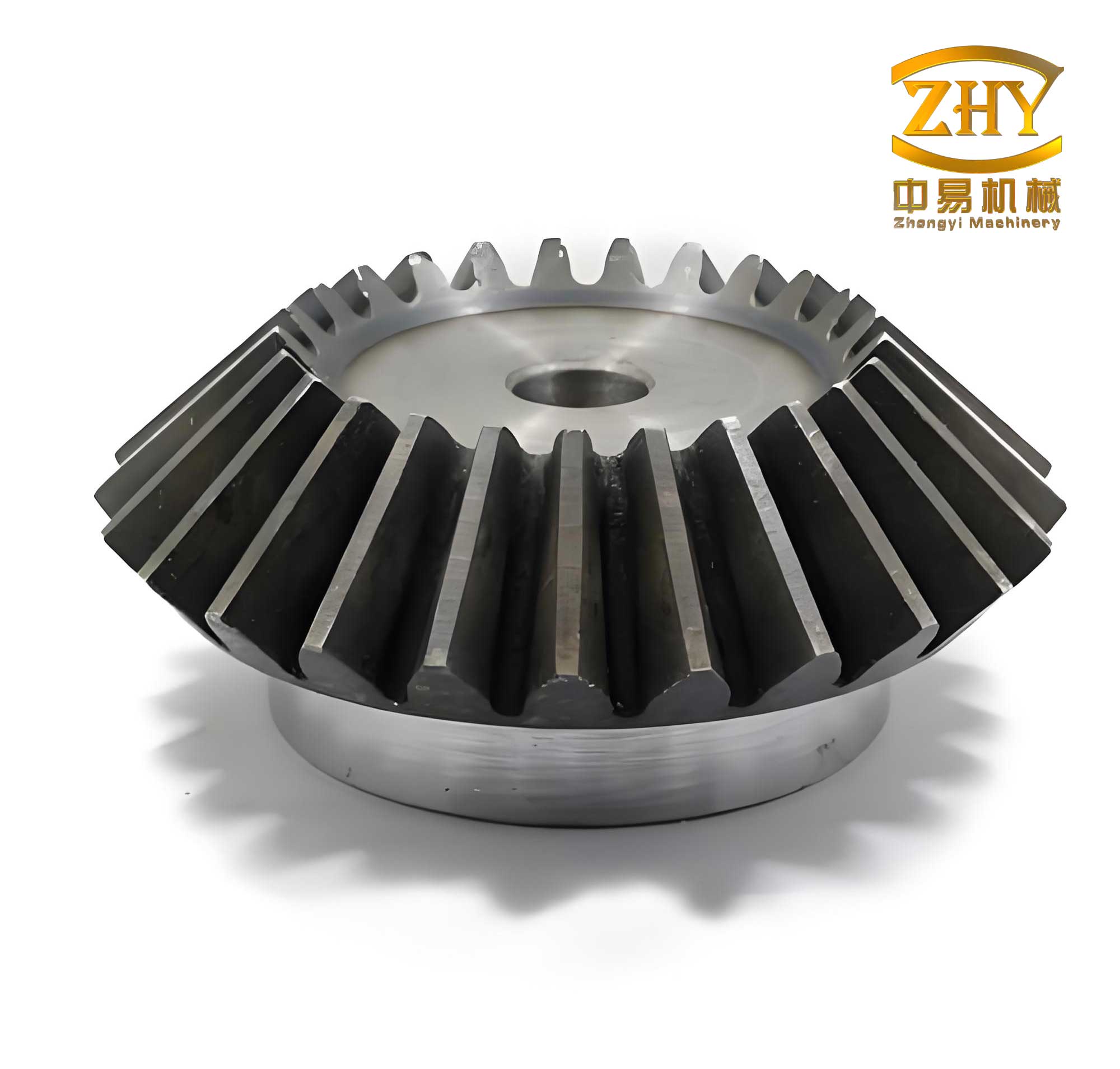
To accurately compute the time-varying meshing stiffness for straight bevel gears, I propose a “slicing method” that overcomes the limitations of traditional potential energy methods designed for cylindrical gears. The core idea is to divide the tooth width \(L\) into \(n\) thin slices along the face width direction. Each slice is treated as a spur gear with local geometric parameters, allowing the application of the potential energy method. The total meshing stiffness of the bevel gear pair is then obtained by summing the stiffness contributions from all slices:
$$ k_{\text{bevel}} = \sum_{i=1}^{n} k_{\text{slice}}^i $$
For each slice, the equivalent parameters are derived based on the conical geometry. The key parameters include the cone angle \(\delta\), module \(m_d\), number of teeth \(Z\), pressure angle \(\alpha\), and face width \(L\). The conversion relations for the equivalent spur gear are:
$$ Z_v = \frac{Z}{\cos\delta} $$
$$ d_v^r = \frac{d^r}{\cos\delta} $$
where \(Z_v\) is the virtual number of teeth, \(d_v^r\) is the equivalent pitch diameter at a reference point, and \(d^r\) is the local pitch diameter. The slice thickness \(dl\) is \(L/n\). For a healthy tooth, the stiffness components for a slice include Hertzian contact stiffness \(k_h\), bending stiffness \(k_b\), axial compressive stiffness \(k_a\), shear stiffness \(k_s\), and fillet foundation stiffness \(k_f\). Using the potential energy method, these are calculated as:
$$ \frac{1}{k_b} = \int_{0}^{d_1} \frac{3(R_b – x_r \cos\alpha_1 – x \cos\alpha_1)^2}{2E dl [y_t – \sqrt{\rho_t^2 – (x_t – x_r – x)^2}]^3} dx + \int_{-\alpha_{te}}^{-\alpha_1} \frac{3\{1 + \cos\alpha_1[(\alpha_2 – \alpha) \sin\alpha – \cos\alpha]\}^2 (\alpha_2 – \alpha) \cos\alpha}{2E dl [\sin\alpha + (\alpha_2 – \alpha) \cos\alpha]^3} d\alpha $$
$$ \frac{1}{k_a} = \int_{0}^{d_1} \frac{\sin^2\alpha_1}{2E dl [y_t – \sqrt{\rho_t^2 – (x_t – x_r – x)^2}]} dx + \int_{-\alpha_{te}}^{-\alpha_1} \frac{(\alpha_2 – \alpha) \cos\alpha \sin^2\alpha_1}{2E dl [\sin\alpha + (\alpha_2 – \alpha) \cos\alpha]} d\alpha $$
$$ \frac{1}{k_s} = \int_{0}^{d_1} \frac{1.2(1+\nu) \cos^2\alpha_1}{E dl [y_t – \sqrt{\rho_t^2 – (x_t – x_r – x)^2}]} dx + \int_{-\alpha_{te}}^{-\alpha_1} \frac{1.2(1+\nu) (\alpha_2 – \alpha) \cos\alpha \cos^2\alpha_1}{E dl [\sin\alpha + (\alpha_2 – \alpha) \cos\alpha]} d\alpha $$
$$ k_h = \frac{\pi E dl}{4(1-\nu^2)} $$
$$ \frac{1}{k_f} = \frac{\cos^2\alpha}{E dl} \left[ L^* \left( \frac{u_f}{S_f} \right)^2 + M^* \left( \frac{u_f}{S_f} \right) + P^* \left(1 + Q^* \tan^2\alpha\right) \right] $$
where \(E\) is Young’s modulus, \(\nu\) is Poisson’s ratio, \(\rho_t\) is the fillet radius, and \(L^*, M^*, P^*, Q^*\) are coefficients dependent on gear geometry. The total slice stiffness for a healthy state is:
$$ \frac{1}{k_{\text{slice}}} = \frac{1}{k_h} + \frac{1}{k_{b1}} + \frac{1}{k_{a1}} + \frac{1}{k_{s1}} + \frac{1}{k_{f1}} + \frac{1}{k_{b2}} + \frac{1}{k_{a2}} + \frac{1}{k_{s2}} + \frac{1}{k_{f2}} $$
For a cracked tooth, the stiffness is reduced due to decreased load-bearing capacity. Assuming a crack initiates at the tooth root and propagates along a line at an angle \(\gamma\) to the tooth centerline, the bending and shear stiffnesses are modified. For a crack depth \(q\) and starting point radius \(R_{cs}\), the affected cross-sectional area and moment of inertia change. The modified stiffness expressions for a slice with crack are:
$$ \frac{1}{k_{b,\text{crack}}} = \int_{0}^{d_1} \frac{12(R_b – x_r \cos\alpha_1 – x \cos\alpha_1)^2}{E dl [h_{cs} – q \sin\gamma + y_t – \sqrt{\rho_t^2 – (x_t – x_r – x)^2}]^3} dx + \int_{-\alpha_{te}}^{-\alpha_c} \frac{12\{1 + \cos\alpha_1[(\alpha_2 – \alpha) \sin\alpha – \cos\alpha]\}^2 (\alpha_2 – \alpha) \cos\alpha}{E dl \left[ \frac{h_{cs}}{R_b} – \frac{q}{R_b} \sin\gamma + \sin\alpha + (\alpha_2 – \alpha) \cos\alpha \right]^3} d\alpha + \int_{-\alpha_c}^{-\alpha_1} \frac{3\{1 + \cos\alpha_1[(\alpha_2 – \alpha) \sin\alpha – \cos\alpha]\}^2 (\alpha_2 – \alpha) \cos\alpha}{2E dl [\sin\alpha + (\alpha_2 – \alpha) \cos\alpha]^3} d\alpha $$
$$ \frac{1}{k_{s,\text{crack}}} = \int_{0}^{d_1} \frac{2.4(1+\nu) \cos^2\alpha_1}{E dl [h_{cs} – q \sin\gamma + y_t – \sqrt{\rho_t^2 – (x_t – x_r – x)^2}]} dx + \int_{-\alpha_{te}}^{-\alpha_c} \frac{2.4(1+\nu) (\alpha_2 – \alpha) \cos\alpha \cos^2\alpha_1}{E dl \left[ \frac{h_{cs}}{R_b} – \frac{q}{R_b} \sin\gamma + \sin\alpha + (\alpha_2 – \alpha) \cos\alpha \right]} d\alpha + \int_{-\alpha_c}^{-\alpha_1} \frac{1.2(1+\nu) (\alpha_2 – \alpha) \cos\alpha \cos^2\alpha_1}{E dl [\sin\alpha + (\alpha_2 – \alpha) \cos\alpha]} d\alpha $$
where \(\alpha_c\) is the pressure angle at the crack tip. The total slice stiffness for a cracked state is then:
$$ \frac{1}{k_{\text{slice},\text{crack}}} = \frac{1}{k_h} + \frac{1}{k_{b1,\text{crack}}} + \frac{1}{k_{a1}} + \frac{1}{k_{s1,\text{crack}}} + \frac{1}{k_{f1}} + \frac{1}{k_{b2}} + \frac{1}{k_{a2}} + \frac{1}{k_{s2}} + \frac{1}{k_{f2}} $$
By summing over all slices, the time-varying meshing stiffness for the bevel gear pair under healthy and cracked conditions can be computed as functions of mesh cycle. This approach allows for efficient evaluation of stiffness changes as cracks propagate, which is vital for dynamic response analysis.
To implement the model, I define the geometric and material parameters for a typical helicopter main reducer bevel gear system. The parameters are summarized in the following tables:
| Parameter | Driving Gear | Driven Gear |
|---|---|---|
| Number of Teeth, \(Z\) | 18 | 36 |
| Module, \(m_d\) (mm) | 4.25 | 4.25 |
| Pressure Angle, \(\alpha\) (deg) | 20 | 20 |
| Face Width, \(L\) (mm) | 27.66 | 27.66 |
| Cone Angle, \(\delta\) (deg) | 26.565 | 63.435 |
| Addendum Coefficient, \(h^*_a\) | 1 | 1 |
| Dedendum Coefficient, \(c^*\) | 0.25 | 0.25 |
| Profile Shift Coefficient, \(X\) | 0 | 0 |
| Parameter | Driving Gear | Driven Gear |
|---|---|---|
| Mass, \(m\) (kg) | 1.313 | 3.679 |
| Diameter Moment of Inertia, \(J_d\) (kg·m²) | 7.672×10⁻⁴ | 4.677×10⁻³ |
| Polar Moment of Inertia, \(J_p\) (kg·m²) | 8.270×10⁻⁴ | 7.340×10⁻³ |
| Parameter | Value (N/m or N·s/m) |
|---|---|
| Transverse Bearing Stiffness, \(k_{bx1}, k_{by1}, k_{bx2}, k_{by2}\) | 1.75×10⁸ |
| Axial Bearing Stiffness, \(k_{bz1}, k_{bz2}\) | 2.27×10⁸ |
| Transverse Bearing Damping, \(c_{bx1}, c_{by1}, c_{bx2}, c_{by2}\) | 933 |
| Axial Bearing Damping, \(c_{bz1}, c_{bz2}\) | 2615 |
Using these parameters, I compute the time-varying meshing stiffness for different fault states. I consider a healthy state and six cracked states where the crack depth \(q\) increases from 0.5 mm to 2.5 mm in steps of 0.5 mm, culminating in a broken tooth (complete fracture). The crack is assumed to start at a radius \(R_{cs} = R_r + 0.5\) mm, where \(R_r\) is the root radius, and propagate at \(\gamma = 70^\circ\) relative to the tooth centerline. The number of slices \(n\) is set to 100 after convergence tests, balancing accuracy and computational efficiency.
The computed meshing stiffness curves over one mesh cycle are shown in the following analysis. For healthy bevel gears, the stiffness exhibits typical double-tooth and single-tooth engagement regions, with symmetric patterns during meshing in and out. As the crack deepens, the stiffness decreases progressively, especially in the single-tooth engagement region where the load is borne by one tooth. The reduction is more pronounced as the meshing point moves toward the tooth tip due to longer lever arms. In the broken tooth case, stiffness drops significantly in double-tooth regions and becomes zero in single-tooth regions where the fractured tooth is engaged.
With the time-varying meshing stiffness determined, I simulate the dynamic response of the bevel gear system by solving the nonlinear equations of motion numerically. I use a Runge-Kutta method with time-step integration. The operating conditions are set as follows: driving gear speed of 300 rpm (5 Hz rotational frequency \(f_{b1}\)), driven gear load torque \(T_2 = 32\) N·m, and meshing frequency \(f_{bm} = 90\) Hz. The backlash \(b\) is set to 20 μm, and the transmission error \(e(t)\) is modeled as a sinusoidal function with amplitude 5 μm. I focus on the acceleration response \(\ddot{y}_1\) of the driving gear in the longitudinal direction, as it is sensitive to meshing forces.
The time-domain and frequency-domain results for different fault states are analyzed. Under healthy conditions, the acceleration signal shows periodic oscillations without significant impulses. The frequency spectrum is dominated by the meshing frequency \(f_{bm}\) and its harmonics (e.g., \(2f_{bm}, 3f_{bm}, …\)), with minimal sidebands. For small cracks (\(q \leq 1.0\) mm), the response is similar to healthy conditions, making early detection challenging. However, as the crack deepens to \(q = 1.5\) mm, distinct periodic impulses appear in the time domain, spaced at intervals \(\Delta t = 0.2\) s, corresponding to the driving gear rotational period \(1/f_{b1}\). In the frequency domain, sidebands emerge around the meshing frequency harmonics, spaced by \(f_{b1}\). For example, around \(5f_{bm}\), sidebands at \(5f_{bm} \pm f_{b1}\) become visible. With further crack propagation (\(q = 2.5\) mm) and broken tooth, the impulse amplitudes increase, and sideband magnitudes rise significantly, indicating severe modulation due to the fault.
To quantify the impact, I compute key metrics such as peak acceleration and sideband amplitude ratios. The results demonstrate that the dynamic model effectively captures the fault progression in bevel gears, highlighting the importance of time-varying stiffness in response analysis. The simulation aligns with theoretical expectations: cracks reduce mesh stiffness, causing impacts during meshing that generate vibration modulations at fault-related frequencies.
To validate the model, I conduct experimental tests on a helicopter transmission system diagnostic platform. The setup includes a driving motor, the bevel gear pair, planetary gear stages, and a loading motor. I compare two states: baseline (healthy) and implanted fault (broken tooth on the driving gear). The operating conditions are set to 300 rpm speed and 82.4 N·m load on the driven gear. Vibration data are acquired using accelerometers mounted near the driving gear bearing, with a sampling frequency of 25.6 kHz and duration of 10 seconds.
The experimental acceleration signals are processed to obtain time-domain waveforms and power spectra. In the baseline test, the time-domain signal shows relatively smooth oscillations, while the power spectrum exhibits peaks at the meshing frequency and its harmonics, with low-level sidebands likely due to manufacturing imperfections. For the broken tooth case, the time-domain signal displays clear periodic impulses every 0.2 s, matching the driving gear rotational period. The power spectrum shows enhanced sidebands around \(f_{bm}\) and \(3f_{bm}\), spaced by \(f_{b1}\), consistent with the simulation predictions. The comparison confirms that the proposed dynamic model accurately reproduces the fault features observed in real bevel gear systems.
The agreement between simulation and experiment underscores the model’s utility for fault diagnosis. By incorporating the slicing-based stiffness calculation, the model can predict vibration responses under various damage scenarios, enabling the development of condition monitoring algorithms for helicopter main reducers. Moreover, the model can be extended to study other bevel gear types, such as spiral bevel gears, by adjusting the geometry and load distribution.
In conclusion, I have developed a nonlinear dynamic model for helicopter main reducer bevel gears that integrates bending-torsion-axial couplings and key nonlinearities like backlash and time-varying meshing stiffness. The novel slicing method for stiffness calculation extends the applicability of potential energy methods to straight bevel gears, facilitating efficient evaluation of healthy and faulty states. Simulation results reveal that crack faults in bevel gears lead to stiffness reduction, periodic impulses in time-domain responses, and characteristic sidebands in frequency spectra, with severity increasing with crack depth. Experimental validation on a test rig confirms the model’s accuracy in capturing fault-induced vibrations. This work provides a foundation for advanced health monitoring systems, contributing to improved reliability and safety of helicopter transmission systems. Future research could explore the effects of lubrication, thermal loads, and multi-fault interactions on bevel gear dynamics, further enhancing predictive maintenance capabilities.