
In my research on precision drive systems for aerospace applications, I have focused extensively on strain wave gears, also known as harmonic gear reducers. These components are critical in solar array drive mechanisms (SADA) due to their exceptional characteristics: high torque capacity, compact and lightweight design, low backlash, and a broad range of reduction ratios. However, the reliable operation of strain wave gears over long mission lifespans is challenged by inevitable strength degradation caused by factors like wear, fatigue, and unpredictable load spectra. Traditional optimal design methods often treat reliability statically, neglecting this temporal degradation. This omission can lead to overly optimistic designs that risk failure before the end of their service life. Therefore, in this work, I develop and solve a dynamic reliability-based optimization design (RBOD) model that explicitly incorporates strength degradation using a stochastic process. The goal is to minimize the volume—and thus the mass—of the strain wave gear reducer while ensuring its reliability remains above a specified threshold throughout its operational life, accounting for the progressive weakening of its components.
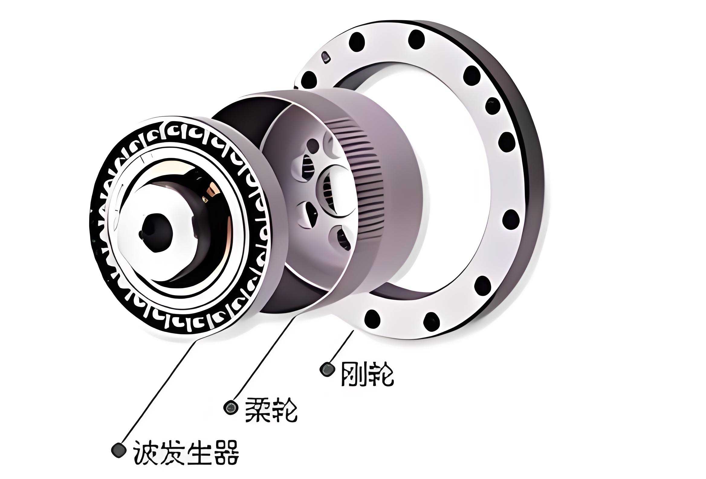
The core of a strain wave gear assembly lies in its three primary components: the wave generator, the flexspline, and the circular spline. The flexspline, a thin-walled cup-shaped component with external teeth, undergoes repeated elastic deformation. This cyclic stressing makes it the most critical element from a fatigue and reliability perspective. Over time, micro-cracks initiate and propagate within the flexspline material due to operational stresses, leading to a gradual reduction in its load-bearing capacity or strength. This phenomenon is what I refer to as strength degradation. Accurately modeling this degradation is paramount for predicting the long-term reliability of the strain wave gear system.
Strength degradation exhibits two key stochastic features: randomness and monotonicity. At any given time, the amount of degradation is not a fixed value but a random variable. Furthermore, degradation is an irreversible process; strength only decreases over time and never increases. Common stochastic processes like Brownian motion or the Wiener process allow for positive and negative increments, making them unsuitable. After analyzing degradation data for mechanical components, I find that the Gamma process is particularly well-suited for modeling slow, monotonic degradation, which is typical for the fatigue-driven strength loss in a strain wave gear’s flexspline.
A Gamma process is a stochastic process with independent, non-negative increments, where each increment follows a Gamma distribution. Let \( D(t) \) represent the cumulative strength degradation at time \( t \). The Gamma process has the following properties:
- \( D(0) = 0 \).
- For \( t > s \ge 0 \), the increment \( \Delta D = D(t) – D(s) \) is independent of the history of the process.
- \( \Delta D \sim \Gamma(\alpha(t) – \alpha(s), \beta) \), meaning it follows a Gamma distribution with shape parameter \( \alpha(t)-\alpha(s) \) and scale parameter \( \beta \).
The probability density function of a Gamma distribution for a random variable \( X \) is:
$$ f(x; \alpha, \beta) = \frac{\beta^{\alpha}}{\Gamma(\alpha)} x^{\alpha-1} e^{-\beta x} I_{(0, \infty)}(x) $$
where \( \alpha > 0 \) is the shape parameter, \( \beta > 0 \) is the scale parameter, \( \Gamma(\cdot) \) is the Gamma function, and \( I(\cdot) \) is the indicator function. For modeling strength degradation, the residual strength \( S(t) \) at time \( t \) can be expressed as the initial strength \( S_0 \) minus the degradation \( D(t) \): \( S(t) = S_0 – D(t) \). The shape function \( \alpha(t) \) is often chosen as a power law or linear function of time, e.g., \( \alpha(t) = c t^b \) or \( \alpha(t) = a t \), depending on the degradation mechanism.
To formulate the dynamic RBOD model for the strain wave gear, I first define the design variables, objective function, and constraints. The primary goal for a SADA application is mass minimization, which translates directly to minimizing the volume of the flexspline, as it is a major contributor to the overall size and weight. The design variables I consider are key geometric parameters of the flexspline:
| Symbol | Description | Unit |
|---|---|---|
| \( d_1 = m \) | Module of the flexspline teeth | mm |
| \( d_2 = l \) | Length of the flexspline cup (smooth barrel section) | mm |
| \( d_3 = \delta \) | Wall thickness of the flexspline toothed rim | mm |
| \( d_4 = b \) | Face width (or tooth width) of the flexspline | mm |
Thus, the design vector is \( \mathbf{d} = [m, l, \delta, b]^T = [d_1, d_2, d_3, d_4]^T \).
The objective function is the volume \( V \) of the flexspline. Based on its geometry—a thin-walled cup with a toothed rim—the volume can be derived as a function of the design variables and other fixed parameters:
$$ V(\mathbf{d}) = \pi b \left[ d_r + (2h_a^* + c^*)m + \delta \right] \left[ (2h_a^* + c^*)m + \delta \right] + 0.816 \pi \delta (l – b) \left[ 1.044 m z_1 – 2(h_a^* + c^*)m + \delta \right] $$
where \( d_r \) is the inner diameter of the flexspline cup, \( h_a^* \) is the addendum coefficient, \( c^* \) is the bottom clearance coefficient, \( z_1 \) is the number of teeth on the flexspline, and other terms relate to the neutral line diameter and wall thickness coefficients. Minimizing \( V(\mathbf{d}) \) is the objective.
The constraints ensure the strain wave gear meets performance, geometric, and reliability criteria. They are formulated as probabilistic constraints because many parameters involved, such as material properties, loads, and stress concentrations, are random in nature. Furthermore, some parameters, like certain correction factors, may have bounds and are treated as interval variables. Let \( \mathbf{x} \) denote the vector of random variables (e.g., material fatigue limits, load torque) and \( \mathbf{y} \) denote the vector of interval variables (e.g., stress concentration factors, load distribution factors). A general probabilistic constraint is expressed as:
$$ \text{Pr} \left\{ g_i(\mathbf{d}, \mathbf{x}, \mathbf{y}) \ge 0 \right\} \ge R_{i, \text{min}} $$
where \( g_i(\cdot) \ge 0 \) represents a performance or state function (e.g., stress less than strength, geometric non-interference), and \( R_{i, \text{min}} \) is the minimum required reliability for that constraint, often set at 0.98 or higher for critical aerospace components.
For the strain wave gear, I consider multiple constraint categories, which I summarize in the following table. The detailed formulation of each \( g_i \) involves complex gear mechanics and elasticity theory.
| Constraint Category | State Function \( g_i \) (Simplified Representation) | Minimum Reliability \( R_{i,\text{min}} \) |
|---|---|---|
| 1. Flexspline Fatigue (Bending & Shear) | \( g_1 \): Calculated cyclic stress < Degraded fatigue strength | 0.98 |
| 2. Load Capacity (Tooth Surface Durability) | \( g_2 \): Contact pressure < Allowable pressure | 0.98 |
| 3. Rim Wall Thickness Limit | \( g_3 \): \( \delta \) ≥ Minimum required for stiffness/strength | 0.98 |
| 4. Bending Strength at Tooth Root | \( g_4 \): Bending stress < Allowable bending stress | 0.98 |
| 5. Flexspline Buckling Stability | \( g_5 \): Critical buckling load > Applied load | 0.98 |
| 6. Cup Length Proportionality | \( g_6 \): \( l \) within limits relative to \( m, z_1 \) | 0.98 |
| 7-11. Geometric & Mesh Constraints | \( g_7\)-\( g_{11} \): Non-interference, proper meshing depth, radial clearance, tip sharpness, etc. | 0.98 |
| 12-21. Dimensional Bounds | \( g_{12}\)-\( g_{21} \): Practical limits on \( m, l, \delta, b \) (e.g., \( 0.3 \le m \le 1.0 \), \( 0.01m z_1 \le \delta \le 0.03 m z_1 \)) | 0.98 |
The most critical constraint is the fatigue constraint \( g_1 \), which directly incorporates strength degradation. For a static reliability model, this constraint compares the maximum induced stress \( \sigma_{\text{max}} \) (a function of \( \mathbf{d}, \mathbf{x}, \mathbf{y} \)) with the initial material fatigue strength \( S_0 \) (a random variable). The reliability is \( R_s = \text{Pr}\{ S_0 > \sigma_{\text{max}} \} \).
For the dynamic model, the strength degrades over time. Let \( S(t) = S_0 – D(t) \), where \( D(t) \) follows a Gamma process with parameters chosen to fit the degradation behavior of the flexspline material (e.g., high-strength alloy steel). The time-dependent reliability at mission time \( t \) is then:
$$ R(t) = \text{Pr}\{ S(t) > \sigma_{\text{max}} \} = \text{Pr}\{ S_0 – D(t) > \sigma_{\text{max}} \} $$
Assuming \( S_0 \) and \( D(t) \) are independent, and given the distribution of \( D(t) \), this probability can be evaluated, often requiring numerical integration or simulation.
The full dynamic RBOD model for the strain wave gear can now be stated. The objective is to minimize volume subject to reliability constraints that are now functions of time. For a target service life of \( T \) years with a minimum reliability \( R_{\text{req}}(T) \) at time \( T \), the optimization problem is:
$$
\begin{aligned}
& \underset{\mathbf{d}, \mathbf{x}, \mathbf{y}}{\text{minimize}}
& & V(\mathbf{d}) \\
& \text{subject to}
& & \text{Pr}\{ g_1(\mathbf{d}, \mathbf{x}, \mathbf{y}, t) = S(t) – \sigma_{\text{max}}(\mathbf{d}, \mathbf{x}, \mathbf{y}) \ge 0 \} \ge R_{\text{req}}(t), \quad \text{for } t \in [0, T] \\
& & & \text{Pr}\{ g_i(\mathbf{d}, \mathbf{x}, \mathbf{y}) \ge 0 \} \ge 0.98, \quad \text{for } i = 2, 3, \ldots, 21.
\end{aligned}
$$
In practice, ensuring reliability over the entire interval can be simplified by enforcing it at the end of life \( t=T \), as reliability is monotonically decreasing. Therefore, a key constraint becomes \( R(T) \ge R_{\text{req}}(T) \). This implies that the initial strength \( S_0 \) must be high enough to compensate for the expected degradation over \( T \) years.
To solve this optimization problem, I employ a nested strategy. The outer loop handles the optimization of design variables \( \mathbf{d} \). For each candidate \( \mathbf{d} \), the inner loop evaluates the reliability constraints, which involves dealing with random variables \( \mathbf{x} \) and interval variables \( \mathbf{y} \). For probabilistic constraints with random variables, I use the First Order Reliability Method (FORM) or Monte Carlo Simulation (MCS) integrated within the optimization routine. Interval variables are handled by considering the worst-case scenario within their bounds, ensuring robustness. The strength degradation via Gamma process is integrated into the reliability assessment for constraint \( g_1 \). I implement this entire framework using MATLAB, leveraging its optimization toolbox (e.g., `fmincon`) for the outer loop and custom functions for reliability analysis.
For a concrete case study, I consider a strain wave gear for a SADA with a required service life of \( T = 5 \) years. The minimum allowable reliability at \( T=5 \) years is set to \( R_{\text{req}}(5) = 0.92 \). The strength degradation of the flexspline’s bending fatigue limit is modeled as a Gamma process with a linear shape function \( \alpha(t) = a t \) and scale parameter \( \beta \). Based on material degradation data, I assume an average degradation rate such that the mean strength decreases by approximately 0.02×10⁸ MPa over 5 years. The initial fatigue strength \( S_0 \) is a random variable following a Weibull distribution. Other random variables include the input torque (normal distribution), material properties (log-normal), etc. Interval variables cover factors like the stress concentration factor \( K_{\sigma} \) which may vary between 1.1 and 1.3 due to manufacturing tolerances.
I solve two models: the traditional static RBOD model (ignoring degradation, requiring \( R(0) \ge 0.92 \)) and the dynamic RBOD model (requiring \( R(5) \ge 0.92 \)). The optimization results for the key design variables and the achieved volume are compared below.
| Design Variable / Result | Static RBOD Model (No Degradation) | Dynamic RBOD Model (With Gamma Process Degradation) |
|---|---|---|
| Module, \( m \) (mm) | 0.8 | 0.8 |
| Cup Length, \( l \) (mm) | 154.8 | 156.7 |
| Tooth Face Width, \( b \) (mm) | 27.1 | 27.1 |
| Rim Wall Thickness, \( \delta \) (mm) | 1.94 | 1.96 |
| Calculated Flexspline Volume, \( V \) (mm³) | 2,689,167.95 | 2,698,268.89 |
| Implied Initial Reliability \( R(0) \) | ≥ 0.92 | ≥ 0.98 |
The results clearly show that the dynamic model yields a more conservative design. While the module \( m \) and face width \( b \) remain identical, the cup length \( l \) and wall thickness \( \delta \) are slightly larger in the dynamic design. This results in a modest increase of about 0.34% in the flexspline volume. The conservatism stems from the reliability requirement. For the static model, it is sufficient to have an initial reliability of 0.92. However, for the dynamic model, to ensure that reliability does not fall below 0.92 after 5 years of strength degradation, the initial system must be significantly more reliable—in this case, with an initial reliability of approximately 0.98. This higher initial reliability is achieved by increasing certain dimensions, making the strain wave gear more robust from the start to accommodate future weakening.
To illustrate the time-dependent reliability profile, I calculate the reliability at each year for the optimal design from the dynamic model, assuming the degradation process holds. The results are plotted in the table below, showing a monotonically decreasing reliability.
| Service Time, \( t \) (years) | Reliability, \( R(t) \) |
|---|---|
| 0 (Initial) | 0.9800 |
| 1 | 0.9705 |
| 2 | 0.9599 |
| 3 | 0.9480 |
| 4 | 0.9347 |
| 5 | 0.9200 |
The mathematical relationship can be fitted, showing an exponential-like decay due to the Gamma process. This curve is crucial for lifecycle management and maintenance planning of the solar array drive mechanism.
The superiority of the dynamic approach becomes evident when considering the actual operational life of the strain wave gear. A design based solely on static reliability might have a 0.92 probability of surviving the initial load conditions. However, as strength degrades, the probability of failure within 5 years would be much higher than the allowable 8% (1-0.92). In contrast, the dynamically optimized strain wave gear is designed with the degradation trajectory in mind, ensuring the reliability target is met at the end of the design life, not just the beginning. This is essential for long-duration space missions where repair or replacement is prohibitively expensive or impossible.
In conclusion, my work demonstrates the critical importance of incorporating time-dependent strength degradation into the reliability-based optimization design of strain wave gears for high-reliability applications like solar array drive assemblies. Using a Gamma process to model the gradual deterioration of the flexspline’s fatigue strength provides a realistic stochastic framework. The resulting dynamic RBOD model yields more conservative and, ultimately, safer designs compared to traditional static methods. The slight increase in material volume or mass is a justified trade-off for guaranteed long-term performance and risk mitigation. For future work, integrating more complex degradation models that account for variable amplitude loading or different failure modes of the strain wave gear could further enhance the design fidelity. Furthermore, multi-objective optimization considering cost, volume, and reliability simultaneously could provide a richer set of design alternatives for engineers. Ultimately, this methodology ensures that the exceptional benefits of strain wave gear technology—high reduction ratios, precision, and compactness—are not compromised by unforeseen in-service degradation, securing the reliable operation of critical aerospace mechanisms for their entire mission lifespan.