
In modern naval architecture, the propulsion system serves as the heart of a vessel, directly influencing its combat effectiveness, survivability, and maneuverability. The ability to maintain stable operation and deliver required thrust across a wide range of rotational speeds, adapting to various sailing conditions and high机动性 demands, is a critical feature and a key technical指标 in the design of marine propulsion systems. Among various propulsion technologies, the dual-cylinder turbine (DCT) propulsion system stands out due to its high power density, long service life, compact structure, operational reliability, and convenient speed regulation. Consequently, it has been adopted by numerous nations as the primary power source for large and ultra-large naval vessels. This study delves into the dynamic characteristics of the herringbone gear system within such a DCT propulsion system, particularly under the influence of unsymmetrical load inputs—a prevalent operational condition that poses significant challenges to system stability.
The operational profile of a DCT propulsion system is complex. During low-speed sailing, the propeller-shaft system is primarily driven by the high-pressure cylinder, while the low-pressure cylinder, due to insufficient steam expansion capability, contributes minimally, leaving its rotor in a follower state. As the vessel accelerates, the low-pressure cylinder rotor transitions from a power-consuming follower to an active power contributor, guided by the reduction gearbox. During high-speed cruising, the power from the low-pressure cylinder increases, approaching that of the high-pressure cylinder, and both cylinders jointly drive the propeller-shaft system through the reduction gears. Full-scale experiments have indicated that this unsymmetrical power input profoundly affects system stability. Issues such as gear tooth impacts and elevated noise levels have emerged as critical bottlenecks hindering the efficient and reliable operation of such propulsion systems. On one hand, as the load ratio between the two cylinders increases, the gear pair on the low-pressure cylinder power transmission chain shifts from a power-consuming state to an active driving state, triggering instability. On the other hand, the coupling of multiple nonlinear factors in such a complex system reduces the predictability of its dynamic response, leading to alternating states of normal tooth meshing, tooth separation, and back-side tooth contact.
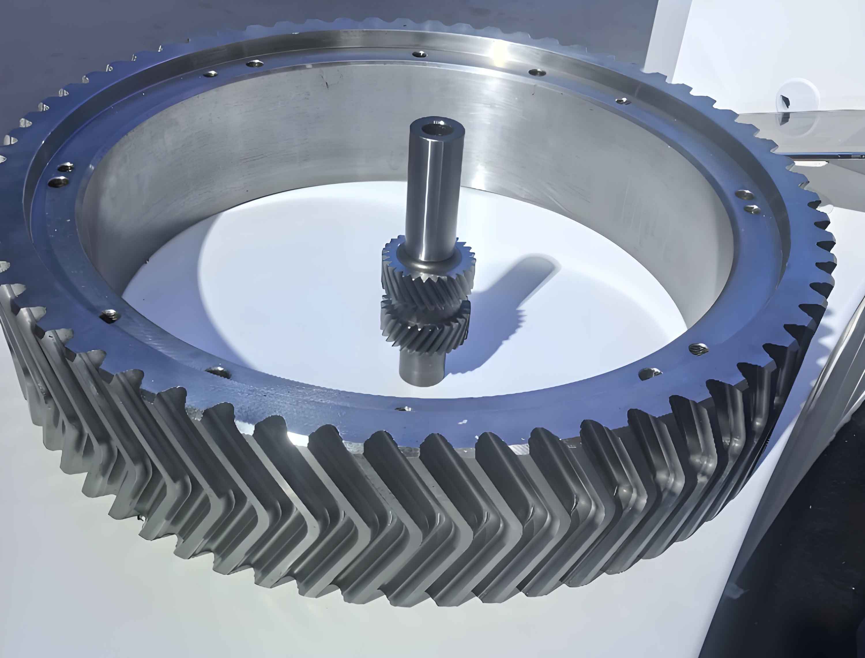
While extensive research exists on the dynamics of general gear transmission systems, studies specifically addressing the nonlinear instability mechanisms of herringbone gear systems under unsymmetrical load inputs are scarce. Therefore, this research focuses on the practical engineering problem of instability in DCT propulsion systems. Based on gear transmission principles and elastohydrodynamic lubrication (EHL) theory for non-Newtonian fluids, we establish a pure torsional dynamic model for a two-stage herringbone gear system. The model incorporates several nonlinear factors, including nonlinear tooth surface friction, nonlinear tooth backlash, and time-varying mesh stiffness. This model is then used to investigate the instability mechanisms and the evolution of dynamic characteristics with system parameters under unsymmetrical load conditions.
The herringbone gear, with its characteristic double-helical structure, offers advantages such as high load capacity, smooth operation, and axial force cancellation, making it ideal for high-power marine transmissions. However, its dynamic behavior becomes significantly more complex under non-ideal loading conditions. In our study, we consider a system where two input shafts (from the high- and low-pressure turbines) drive a common output shaft (connected to the propeller) through a two-stage herringbone gear reduction unit. The dynamic model focuses on the torsional vibrations of the gears, neglecting lateral and axial vibrations to simplify the analysis while capturing the essential nonlinear phenomena.
The governing equations of motion for the herringbone gear system are derived using Lagrange’s equation. The system comprises several inertias: the high-pressure turbine rotor (Ihp), the low-pressure turbine rotor (Ilp), the pinions and gears of the two stages, and the propeller load (Ip). The equations account for the gear mesh forces, damping, and the external input torques. The key nonlinearities are modeled as follows:
Time-Varying Mesh Stiffness: The mesh stiffness of a herringbone gear pair varies periodically with the gear rotation due to the changing number of tooth pairs in contact and the elastic deflection of the teeth. For a single helical gear, the mesh stiffness can be approximated by a Fourier series. For the herringbone gear, the combined stiffness from the two helices is considered. The time-varying mesh stiffness for the first-stage gear pair, \( k_{m1}(t) \), and the second-stage pair, \( k_{m2}(t) \), are given by:
$$ k_{m1}(t) = k_{m1,avg} + \sum_{n=1}^{N} a_{n1} \cos(n \omega_{m1} t + \phi_{n1}) $$
$$ k_{m2}(t) = k_{m2,avg} + \sum_{n=1}^{N} a_{n2} \cos(n \omega_{m2} t + \phi_{n2}) $$
where \( k_{m,avg} \) is the average mesh stiffness, \( a_n \) are the Fourier coefficients, \( \omega_m \) is the mesh frequency, and \( \phi_n \) are phase angles. The mesh frequency is related to the rotational speed and the number of teeth: \( \omega_m = Z \omega \), where \( Z \) is the number of teeth and \( \omega \) is the angular velocity of the gear.
Nonlinear Tooth Backlash: The backlash function, \( f(\delta) \), where \( \delta \) is the relative displacement between meshing teeth along the line of action, is modeled as a piecewise linear function:
$$ f(\delta) =
\begin{cases}
\delta – b, & \text{if } \delta > b \\
0, & \text{if } |\delta| \le b \\
\delta + b, & \text{if } \delta < -b
\end{cases} $$
Here, \( 2b \) represents the total backlash. This nonlinearity introduces discontinuities in the system, leading to impacts during tooth separation and re-engagement.
Nonlinear Tooth Surface Friction: The friction force on the tooth surface, which acts perpendicular to the line of action, is modeled based on elastohydrodynamic lubrication conditions. The friction coefficient \( \mu \) is a function of the slide-to-roll ratio (SRR), contact pressure, and lubricant properties. A simplified model is used:
$$ F_f = \mu(\lambda) \cdot F_n $$
$$ \mu(\lambda) = \mu_0 \cdot \text{sgn}(v_s) \cdot \left(1 – e^{-\alpha |v_s|}\right) $$
where \( F_n \) is the normal contact force, \( v_s \) is the sliding velocity, \( \mu_0 \) is the maximum friction coefficient, and \( \alpha \) is a constant. This friction force introduces additional damping and nonlinear excitation into the system.
Elastohydrodynamic Lubrication (EHL) Influence: The lubricant film between meshing teeth affects the contact stiffness and damping. The EHL film thickness influences the effective mesh stiffness. A simplified model incorporates a damping term \( c_{ehl} \) proportional to the film thickness and the relative velocity.
The complete set of nonlinear differential equations for the torsional dynamics of the two-stage herringbone gear system can be summarized as follows. Let \( \theta_i \) and \( I_i \) represent the angular displacement and moment of inertia for the i-th component. The equations for the high-pressure input shaft (1), low-pressure input shaft (2), first-stage pinion (3), first-stage gear (4), second-stage pinion (5), second-stage gear (6), and output propeller shaft (7) are:
$$ I_1 \ddot{\theta}_1 = T_{hp} – R_{p1} \left[ k_{m1}(t) f(\delta_1) + c_{m1} \dot{\delta}_1 \right] – R_{p1} F_{f1} $$
$$ I_2 \ddot{\theta}_2 = T_{lp} – R_{p2} \left[ k_{m1}(t) f(\delta_1′) + c_{m1} \dot{\delta}_1′ \right] – R_{p2} F_{f1}’ $$
$$ I_3 \ddot{\theta}_3 = R_{p1} \left[ k_{m1}(t) f(\delta_1) + c_{m1} \dot{\delta}_1 \right] + R_{p1} F_{f1} – R_{p3} \left[ k_{m2}(t) f(\delta_2) + c_{m2} \dot{\delta}_2 \right] – R_{p3} F_{f2} $$
$$ I_4 \ddot{\theta}_4 = R_{g1} \left[ k_{m1}(t) f(\delta_1′) + c_{m1} \dot{\delta}_1′ \right] + R_{g1} F_{f1}’ – R_{p4} \left[ k_{m2}(t) f(\delta_2′) + c_{m2} \dot{\delta}_2′ \right] – R_{p4} F_{f2}’ $$
$$ I_5 \ddot{\theta}_5 = R_{p3} \left[ k_{m2}(t) f(\delta_2) + c_{m2} \dot{\delta}_2 \right] + R_{p3} F_{f2} $$
$$ I_6 \ddot{\theta}_6 = R_{p4} \left[ k_{m2}(t) f(\delta_2′) + c_{m2} \dot{\delta}_2′ \right] + R_{p4} F_{f2}’ $$
$$ I_7 \ddot{\theta}_7 = R_{g2} \left[ k_{m2}(t) f(\delta_2) + c_{m2} \dot{\delta}_2 \right] + R_{g2} F_{f2} – T_{load} $$
Here, \( T_{hp} \) and \( T_{lp} \) are the input torques from the high-pressure and low-pressure cylinders, respectively. \( T_{load} \) is the propeller load torque. \( R_{pi} \) and \( R_{gi} \) are the base radii of pinions and gears. The relative displacements \( \delta_1, \delta_1′, \delta_2, \delta_2′ \) are defined based on the angular displacements and base radii. For example, \( \delta_1 = R_{p1} \theta_1 – R_{g1} \theta_4 – e_1(t) \), where \( e_1(t) \) is the static transmission error for the first-stage herringbone gear pair, often modeled as a sinusoidal function. The friction forces \( F_{f1}, F_{f1}’, F_{f2}, F_{f2}’ \) are calculated using the friction model described earlier.
To analyze the system’s behavior under unsymmetrical loads, we define the load ratio \( \gamma = T_{lp} / T_{hp} \) and the total load level \( T_{total} = T_{hp} + T_{lp} \). The dynamic response is studied as these parameters vary. We employ numerical integration techniques, such as the Runge-Kutta method, to solve the nonlinear equations of motion over time.
To quantify the system’s dynamic characteristics and stability, we propose three evaluation indicators:
1. Stability Indicator (LE): The largest Lyapunov exponent, calculated from the time series data of the system’s response. A positive LE indicates chaotic behavior, while a zero or negative LE suggests periodic or quasi-periodic motion.
2. Amplitude Indicator (Am): The peak-to-peak amplitude of the torsional vibration of a key component, such as the low-pressure side gear, normalized by the nominal static deflection.
3. Impact Time Ratio (ζ): The ratio of time spent in back-side contact (impact) to the total time in a given period. This indicator reflects the severity of tooth separation and collisions.
The calculation of these indicators for various operational points allows us to map the system’s behavior across the parameter space. The parameters used in the simulation are based on a typical marine herringbone gear reduction unit. A representative set of system parameters is listed in the table below.
| Parameter | Symbol | Value | Unit |
|---|---|---|---|
| Moment of Inertia, High-Pressure Turbine | \( I_{hp} \) | 15.0 | kg·m² |
| Moment of Inertia, Low-Pressure Turbine | \( I_{lp} \) | 18.0 | kg·m² |
| Moment of Inertia, 1st Stage Pinion | \( I_{p1} \) | 0.8 | kg·m² |
| Moment of Inertia, 1st Stage Gear | \( I_{g1} \) | 5.2 | kg·m² |
| Moment of Inertia, 2nd Stage Pinion | \( I_{p2} \) | 2.5 | kg·m² |
| Moment of Inertia, 2nd Stage Gear | \( I_{g2} \) | 22.0 | kg·m² |
| Moment of Inertia, Propeller | \( I_{prop} \) | 250.0 | kg·m² |
| Number of Teeth, 1st Stage Pinion | \( Z_{p1} \) | 25 | – |
| Number of Teeth, 1st Stage Gear | \( Z_{g1} \) | 80 | – |
| Number of Teeth, 2nd Stage Pinion | \( Z_{p2} \) | 30 | – |
| Number of Teeth, 2nd Stage Gear | \( Z_{g2} \) | 100 | – |
| Average Mesh Stiffness, 1st Stage | \( k_{m1,avg} \) | 1.2e8 | N/m |
| Average Mesh Stiffness, 2nd Stage | \( k_{m2,avg} \) | 2.5e8 | N/m |
| Mesh Damping Ratio | \( \zeta_m \) | 0.07 | – |
| Backlash, 1st Stage | \( 2b_1 \) | 40 | µm |
| Backlash, 2nd Stage | \( 2b_2 \) | 50 | µm |
| Base Radius, 1st Stage Pinion | \( R_{p1} \) | 0.075 | m |
| Base Radius, 1st Stage Gear | \( R_{g1} \) | 0.240 | m |
| Base Radius, 2nd Stage Pinion | \( R_{p2} \) | 0.090 | m |
| Base Radius, 2nd Stage Gear | \( R_{g2} \) | 0.300 | m |
| Helix Angle | \( \beta \) | 25 | ° |
The herringbone gear’s helix angle is crucial as it determines the axial force balance and the effective contact line length. The double-helical design of the herringbone gear inherently cancels axial forces, but under unsymmetrical loading, the load distribution between the two helices may become uneven, affecting the mesh stiffness and dynamics. This effect is incorporated into the time-varying stiffness model by considering the phase difference between the meshing on the two helices.
Through extensive numerical simulations, we investigate the system’s response for different combinations of the load ratio \( \gamma \) and the total load level \( T_{total} \). The high-pressure input torque \( T_{hp} \) is varied from 5 kNm to 50 kNm, and the load ratio \( \gamma \) from 0.1 to 1.2. The results, characterized by the three indicators, reveal distinct dynamic regimes. We can categorize the parameter space into three control regions:
Control Region I: This region corresponds to low load ratios (typically \( \gamma < 0.4 \)) and moderate total loads. In this regime, the gear pair on the low-pressure side operates predominantly in back-side contact (背啮). The dynamic response is predominantly periodic, with small vibration amplitudes and smooth operation. The Lyapunov exponent (LE) is near zero or slightly negative, indicating limit cycle behavior. The amplitude indicator (Am) is low, often below 2.0 (normalized). The impact time ratio (ζ) is relatively high, as the low-pressure side gear is lightly loaded and tends to rattle within the backlash. However, due to the low forces, these impacts are not severe. The herringbone gear system exhibits stable and predictable dynamics in this region.
| Indicator | Value | Interpretation |
|---|---|---|
| Largest Lyapunov Exponent (LE) | -0.02 | Periodic motion |
| Amplitude Indicator (Am) | 1.5 | Low vibration level |
| Impact Time Ratio (ζ) | 0.65 | High proportion of back-side contact |
Control Region II: As the load ratio increases (e.g., \( 0.4 < \gamma < 0.8 \)) for a given total load, the system undergoes a sudden transition. The motion becomes highly irregular, exhibiting characteristics of chaos. The Lyapunov exponent becomes positive, confirming chaotic behavior. The vibration amplitudes increase dramatically, often exceeding 5 times the normalized value. Interestingly, the impact time ratio (ζ) decreases compared to Region I because the increased load on the low-pressure side pushes the gear pair towards the normal operating flank, reducing back-side contact time. However, when impacts do occur, they are more severe due to the higher kinetic energy involved. This region represents an instability zone where the herringbone gear system experiences large, unpredictable vibrations, posing risks of excessive noise, wear, and potential failure.
| Indicator | Value | Interpretation |
|---|---|---|
| Largest Lyapunov Exponent (LE) | +0.15 | Chaotic motion |
| Amplitude Indicator (Am) | 5.8 | High vibration level |
| Impact Time Ratio (ζ) | 0.35 | Moderate back-side contact |
Control Region III: For even higher load ratios ( \( \gamma > 0.8 \) ), approaching symmetric loading (\( \gamma = 1 \)), the system dynamics undergo another abrupt change. The motion returns to a more ordered state, but not necessarily periodic. It may be quasi-periodic or a complex multi-periodic motion. The Lyapunov exponent drops to near zero or becomes slightly negative again. The vibration amplitude decreases significantly from the peaks in Region II but may remain higher than in Region I. The impact time ratio (ζ) becomes very low, as both input shafts are actively driving the system, minimizing tooth separation. The herringbone gear system operates in a relatively stable manner in this region, though the dynamic response is sensitive to parameter variations near the boundary with Region II.
| Indicator | Value | Interpretation |
|---|---|---|
| Largest Lyapunov Exponent (LE) | -0.01 | Quasi-periodic motion |
| Amplitude Indicator (Am) | 2.2 | Moderate vibration level |
| Impact Time Ratio (ζ) | 0.10 | Low back-side contact |
The transition between these regions is not solely dependent on the load ratio \( \gamma \); it also interacts with the total load level \( T_{total} \). To visualize this interaction, we can define a composite parameter, such as the effective unbalance parameter \( \eta = \gamma \cdot \sqrt{T_{total}/T_{ref}} \), where \( T_{ref} \) is a reference torque. The boundaries between the control regions can be approximated by critical values of \( \eta \). For the studied herringbone gear system, the approximate boundaries are:
$$ \eta_{I-II} \approx 0.25 $$
$$ \eta_{II-III} \approx 0.55 $$
These boundaries provide a practical guideline for system design and operation. The physical interpretation is that instability arises when the load on the previously follower low-pressure side becomes significant enough to actively participate in power transmission but not enough to establish stable, symmetric load sharing. The nonlinearities, particularly the backlash and time-varying stiffness, interact to produce complex bifurcations and chaos in this transitional regime.
The influence of other design parameters of the herringbone gear on these dynamic regions is also significant. For instance, the helix angle \( \beta \) affects the overlap ratio and the axial coupling between the two helices. A larger helix angle increases the overlap, leading to smoother transmission and potentially wider stable regions. The backlash magnitude directly influences the severity of impacts. Reducing backlash can shrink Region II but may increase contact loads and manufacturing costs. The mesh stiffness fluctuation amplitude, determined by gear design parameters like module and tooth profile, also plays a role. Larger stiffness variations tend to excite parametric resonances, potentially expanding the chaotic Region II.
To further elucidate the system’s behavior, we present a detailed bifurcation analysis. Holding the total load constant at \( T_{total} = 35 \text{ kNm} \), we vary the load ratio \( \gamma \) from 0.1 to 1.2 and compute the Poincaré sections of the angular velocity of the low-pressure side gear. The results show a period-doubling route to chaos as \( \gamma \) enters Region II, and a reverse period-halving route as it exits into Region III. The mathematical representation of the Poincaré map can be complex, but the essence is captured by the following iterative relation derived from the stroboscopic sampling of the periodic forcing component (mesh frequency):
$$ \mathbf{x}_{n+1} = \mathbf{P}(\mathbf{x}_n; \gamma) $$
where \( \mathbf{x}_n \) is the state vector (displacements and velocities) at the n-th Poincaré section, and \( \mathbf{P} \) is the mapping function. The eigenvalues of the linearized map \( D\mathbf{P} \) indicate stability: crossing the unit circle through -1 indicates a period-doubling bifurcation, a signature of the transition into chaos.
The proposed evaluation indicators (LE, Am, ζ) provide a comprehensive, quantitative measure of the herringbone gear system’s health and stability. For practical monitoring, these indicators can be estimated from vibration acceleration signals measured on the gearbox housing using advanced signal processing techniques, such as phase space reconstruction for Lyapunov exponent calculation and envelope analysis for impact detection.
In conclusion, our investigation into the dynamics of herringbone gears within marine dual-cylinder turbine propulsion systems reveals a rich and complex dynamic landscape governed by unsymmetrical load inputs. The herringbone gear system exhibits three distinct dynamic regimes depending on the load ratio and total load level. The intermediate region (Control Region II) is characterized by chaotic motion, large vibration amplitudes, and represents an instability zone that should be avoided in operation. The herringbone gear design, while advantageous for load capacity and smoothness, requires careful consideration of its dynamic response under partial load conditions typical of DCT operation. For system design and optimization, it is advisable to select operational parameters within Control Region I or III, where the dynamics are more predictable and vibration levels are acceptable. This may involve tuning the control logic of the turbine system to avoid prolonged operation in critical load-sharing ratios or modifying the herringbone gear design parameters, such as backlash and mesh stiffness characteristics, to shift the unstable region outside the normal operational envelope. Future work will extend this model to include lateral-torsional-axial coupling vibrations and experimental validation on a test rig to further refine the understanding of herringbone gear dynamics in marine applications.
The robustness of the herringbone gear configuration is thus not inherent but must be ensured through meticulous dynamic analysis and parameter design, highlighting the importance of integrated modeling approaches that account for the multifaceted nonlinearities present in real-world marine propulsion systems.