
1. Introduction and Research Background
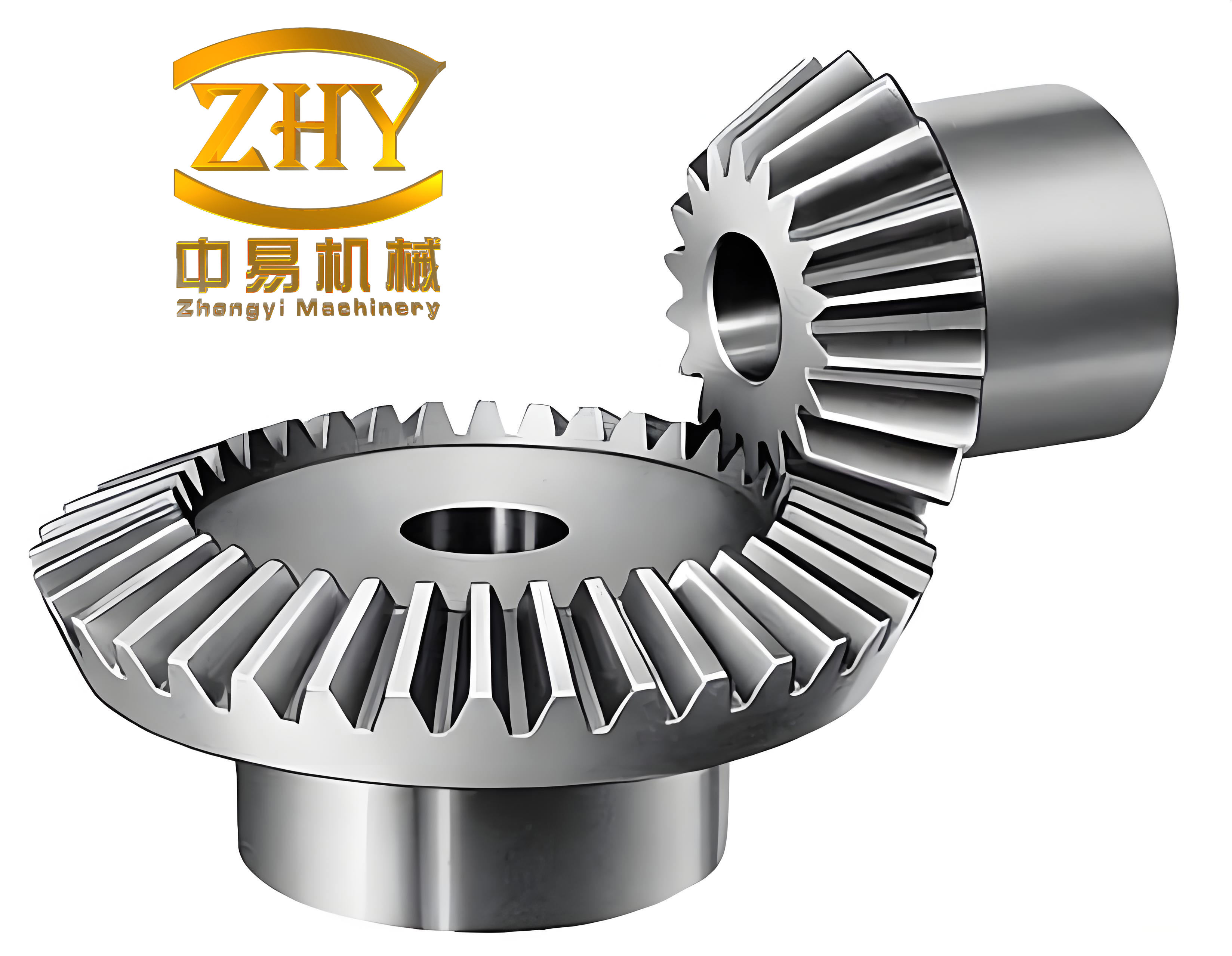
During my research on advanced manufacturing technologies, I have focused on the machining challenges associated with straight bevel gears. Bevel gear transmissions exhibit characteristics such as high load capacity, smooth transmission, and compact structural design, making them essential components in vehicles, marine vessels, machine tools, oil drilling equipment, aerospace applications, and other power-driven systems. In the rapidly evolving landscape of equipment electrification, gears remain irreplaceable as transmission elements within mechanical systems.
Straight bevel gears are commonly manufactured using generative machining methods including gear planing, twin-cutter milling, and circular lapping. These methods offer high processing efficiency but present several drawbacks: specialized machine tool requirements, high procurement costs, difficulty in accommodating large-dimension gears, and they are unsuitable for single-piece or small-batch production. The high flexibility of multi-axis machining centers combined with universal cutting tools provides an alternative solution for addressing small-batch and large-specification bevel gear processing challenges. However, gear machining based on machining centers typically treats the gear tooth surface as a free-form surface, resulting in low material removal rates and difficulties in improving machining efficiency.
Furthermore, most current machining center-based gear manufacturing methods utilize theoretical tooth surfaces with line conjugation as the model. Under load conditions, edge contact phenomena can emerge, leading to premature gear pair failure. This motivated my research to investigate processing methods based on the digital generative principle, aiming to substantially enhance the efficiency of gear machining on machining centers while complementing traditional gear generative machining technologies that employ specialized machine tools.
In response to these challenges, I have proposed a small-batch bevel gear machining method grounded in the digital generative principle. This method utilizes universal cutting tools and their trajectory motion to form a virtual production gear that generates the workpiece gear, thereby preserving generative machining characteristics during tooth surface processing while significantly improving processing efficiency. The following table summarizes the comparative advantages of different machining approaches:
| Machining Method | Efficiency | Flexibility | Tooling Cost | Suitability for Small Batches |
|---|---|---|---|---|
| Traditional Generative Machining | High | Low | High | Poor |
| Machining Center with End Mill | Low | High | Low | Good |
| Digital Generative Machining (Proposed) | High | High | Medium | Excellent |
2. Tooth Surface Equation and Digital Generative Principle
2.1 Production Gear Tooth Surface Construction
In my methodology, the production gear for machining straight bevel gears is a fictitious gear with a pitch cone angle of 90°, whose pitch cone surface becomes a plane. This type of planar production gear is referred to as a crown gear. The meshing between the crown gear and the workpiece gear resembles the engagement between a rack and a spur gear. Based on gear transmission theory and the geometric characteristics of the production gear, I established a similar straight bevel gear generation process. The meshing relationship between the production gear and the workpiece gear is illustrated through the coordinate systems and angular relationships defined in my mathematical derivation.
To begin with, the number of teeth on the production gear can be determined from the transmission ratio relationship. For two intersecting axes Z₁ and Z₂ forming an angle Σ, the instantaneous axis of rotation OI represents the line of action of the angular velocity of gear 1 relative to gear 2:
$$\boldsymbol{\omega}_{12} = \boldsymbol{\omega}_1 – \boldsymbol{\omega}_2 \tag{1}$$
The orientation of OI relative to the gear axes is determined by angles γ₁ and γ₂, representing the pitch cone angles of gears 1 and 2 respectively:
$$\tan \gamma_1 = \frac{\sin \Sigma}{m_{12} + \cos \Sigma} \tag{2}$$
$$\tan \gamma_2 = \frac{\sin \Sigma}{m_{21} + \cos \Sigma} \tag{3}$$
where the relationship between the angles and the transmission ratio is:
$$\Sigma = \gamma_1 + \gamma_2 \tag{4}$$
$$m_{12} = \frac{\omega_1}{\omega_2} = \frac{N_2}{N_1} = \frac{\sin \gamma_2}{\sin \gamma_1} \tag{5}$$
When the shaft angle Σ equals 90°, the above equations simplify to:
$$\tan \gamma_1 = \frac{N_2}{N_1} = \frac{1}{m_{12}} \tag{6}$$
$$\tan \gamma_2 = \frac{N_1}{N_2} = \frac{1}{m_{21}} \tag{7}$$
The shaft angle between the production gear and the machined bevel gear is expressed as:
$$\Sigma = 90° + \gamma_1 \tag{8}$$
For the production gear (crown gear), the base cone angle can be determined from:
$$\gamma_p = \frac{\pi}{2} \tag{9}$$
$$\sin \gamma_b = \frac{\sin \alpha \cdot \sin(\pi/2)}{\sin(90° – \alpha) \cdot \sin(\pi/2)} = 1 \tag{10}$$
which simplifies to:
$$\gamma_b = \frac{\pi}{2} – \alpha \tag{11}$$
where α represents the pressure angle. The three-dimensional geometry of the production gear involves tracking spherical involute profiles projected onto the sphere’s center to determine the production gear tooth surface.
When the production gear tooth surface is planar, the resulting bevel gear tooth profile is known as the figure-8 tooth form. Considering point P on the great circle of a sphere with radius ρ, I defined the production gear tooth surface in coordinate system S₀, where ρ serves as the longitudinal parameter of the production gear tooth surface. By transforming point P coordinates from S₀(x₀, y₀, z₀) to S₃(x₃, y₃, z₃), I obtained the production gear tooth surface expression:
$$\mathbf{r}_{cg}(\rho, \varphi) = \mathbf{M}_{32} \cdot \mathbf{M}_{21} \cdot \mathbf{M}_{10} \cdot \mathbf{r}_P^{(0)}(\rho, \varphi) \tag{12}$$
After performing the coordinate transformations and algebraic simplifications, the production gear tooth surface can be expressed in matrix form:
$$\mathbf{r}_{cg}(\rho, \varphi) = \begin{bmatrix} \rho \cos \varphi \sin(\frac{t_p}{2}) \pm \sin \varphi \sin \alpha \cos(\frac{t_p}{2}) \\ \rho (\cos \varphi \cos(\frac{t_p}{2}) – \sin \varphi \sin \alpha \sin(\frac{t_p}{2})) \\ -\rho \sin \varphi \cos \alpha \\ 1 \end{bmatrix} \tag{13}$$
where t_p denotes the generated gear tooth thickness, given by:
$$t_p = \frac{\pi}{N} \tag{14}$$
The angular parameter φ varies between the root angle and tip angle of the production gear, corresponding to the root angle and tip angle of the generated bevel gear.
2.2 Gear Tooth Surface Equation
I then established the tooth surface equation for the straight bevel gear by considering the meshing relationship between the production gear and the generated gear. The coordinate systems S_cg and S_i are rigidly connected to the production gear and the generated gear (pinion i=1, gear i=2) respectively. The gear tooth surface is determined as the envelope of the family of production gear tooth surfaces in the gear coordinate system S_i:
$$\mathbf{r}_i(\rho, \varphi, \psi_i) = \mathbf{M}_{il} \cdot \mathbf{M}_{lk} \cdot \mathbf{M}_{kj} \cdot \mathbf{M}_{jcg} \cdot \mathbf{r}_{cg}(\rho, \varphi) \tag{15}$$
The normal vector of the gear tooth surface is:
$$\mathbf{n}_i(\rho, \varphi, \psi_i) = \mathbf{M}_{il} \cdot \mathbf{M}_{lk} \cdot \mathbf{M}_{kj} \cdot \mathbf{M}_{jcg} \cdot \mathbf{n}_{cg}(\rho, \varphi) \tag{16}$$
The rotation angles ψ_cg and ψ_i are related through the gear ratio:
$$\psi_{cg} = \frac{N_i}{N_{cg}} \cdot \psi_i \tag{17}$$
Based on the gear meshing theory, a point on the production gear surface can become a point on the generated gear tooth surface through coordinate transformation, provided that the meshing equation is satisfied:
$$\mathbf{R}_V = \mathbf{r}_3 \tag{18}$$
$$\mathbf{V}_{12} = \mathbf{V}_R – \mathbf{V}_{cg} \tag{19}$$
$$\mathbf{n}_V \cdot \mathbf{V}_{12} = 0 \tag{20}$$
Through iterative solving of the meshing equations with the tooth surface parameters, I obtained the discrete digital tooth surface representation. The iterative solving process involves:
$$\begin{cases} \mathbf{r}_i(\rho, \varphi, \psi_i) – L = 0 \\ \mathbf{r}_i(\rho, \varphi, \psi_i) – R = 0 \\ \mathbf{n} \cdot \mathbf{V}_{12} = 0 \end{cases} \tag{21}$$
where L represents the coordinate along the gear axis from the shaft intersection point, and R represents the radius perpendicular to the axis. The iteration process is shown in Table 1:
| Step | Description | Parameters |
|---|---|---|
| 1 | Determine production gear tooth surface point | ρ, φ |
| 2 | Calculate relative velocity | V₁₂ = f(ω_R, ω_cg) |
| 3 | Apply meshing equation | n · V₁₂ = 0 |
| 4 | Solve for tooth surface parameters | ρ, φ, ψ_i |
| 5 | Transform to gear coordinate system | Output tooth surface points |
2.3 The Digital Generative Principle
Traditional tooth surface generative machining methods accomplish generative motion through mechanical transmission mechanisms, but their motion control capabilities are limited. In contrast, the digital generative principle I have proposed leverages the high flexibility of machining center motion. Two reciprocating cutting tools (planing cutters) form the tooth surface of the production gear, and the workpiece performs generative motion with the production gear to machine the straight bevel gear teeth.
In conventional machining, the production gear is typically constructed using a cradle, with tool cutting edge trajectories forming the production gear tooth surface. This production gear tooth surface is a ruled surface that can be formed by sweeping the generatrix of a universal conical or cylindrical end mill on a machining center. At any instantaneous meshing position between the production surface and the workpiece tooth surface, the production surface can be expressed in the workpiece gear coordinate system. As the machining meshing motion progresses, the production surface changes position in the gear coordinate system while the universal tool simultaneously changes position in the production gear coordinate system. The tool’s combined motion produces the discrete digital production surface that meshes with the workpiece tooth surface.
In my proposed method, I first control the universal tool sweep to form a discrete virtual production gear on the machining center, then control the virtual meshing between the virtual production gear and the workpiece gear to generate the gear tooth surface. To further enhance material removal efficiency, I employed relatively larger diameter dovetail disc cutters instead of end mills to sweep the production surface. However, the interference between the cutter and the tooth surface becomes more prominent and must be addressed through careful selection of the disc cutter cone angle, diameter, and control of the cutter posture.
3. Tooth Surface Modification for Straight Bevel Gears
3.1 Modification Principle Analysis
Modern power transmission gears require appropriate tooth surface modification to accommodate system deformation under load and meshing misalignment that can lead to edge contact and degraded meshing performance. To achieve this, I established a comprehensive mathematical model for tooth surface modification by analyzing the completely conjugate theoretical tooth surfaces of the driving and driven gears based on their macro-geometric parameters and transmission conditions. This enabled me to establish the mapping relationship between gear contact characteristic control parameters—including contact reference point position, contact trace direction, instantaneous contact ellipse length, and transmission error curve—and the conjugate difference surface of the gear pair.
3.2 Tooth Length Direction Modification
During gear operation, deformation of gear materials, shafts, and supports occurs due to force transmission, causing axis misalignment of the gear pair. Furthermore, high-speed rotation induces deformation that causes non-uniform contact load distribution across the tooth width. I addressed these issues through tooth length direction modification. Following the parabolic modification approach, the magnitude of modification is defined based on the contact zone length, enabling determination of the parabolic curvature and its equation. The modification amount in the tooth surface normal direction is calculated from the parabolic equation.
Applying the tooth surface formation principle, the instantaneous contact line before modification appears as a straight line during production surface-workpiece gear meshing. The generated gear tooth surface consists of countless instantaneous contact lines. Based on this principle, I performed tooth length direction modification by introducing a parabolic function instead of the straight contact line:
$$y = ax^2 \tag{22}$$
where the coordinate system origin is at the midpoint of the instantaneous contact line, the x-coordinate corresponds to ρ, the y-coordinate corresponds to the modification curve deformation amount, and a is the modification coefficient determined by back-calculation from the preset deformation amount. After modification, any point A(x, y, z) on the contact line transforms to point B(x₁, y₁, z₁):
$$\begin{bmatrix} x_1 \\ y_1 \\ z_1 \end{bmatrix} = \begin{bmatrix} x \\ y \\ z \end{bmatrix} + \Delta \phi \cdot \mathbf{n} \tag{23}$$
where Δφ represents the deformation amount obtained from the parabolic equation, and n represents the normal vector of the tooth surface point.
3.3 Tooth Height Direction Modification
Through the meshing theory analysis, when the virtual production gear generates the workpiece gear tooth surface during their virtual meshing, a constant transmission ratio exists between the production gear rotation angle and the gear rotation angle. I modified the tooth height direction by changing the transmission ratio from constant to instantaneous, converting the constant transmission ratio to an instantaneous rotational ratio:
$$\begin{cases} \Delta \psi = \psi_i^{(0)} – \psi_i \\ \psi_{cg} = \frac{N_i}{N_{cg}} \cdot \psi_i \\ R_{aq}^{(0)} = \frac{N_R}{N_{cg}} \\ \psi_{cg} = \psi_{aq}^{(0)} + \Delta \psi_{aq} \\ \Delta \psi_{aq} = b \cdot \Delta \psi^2 \end{cases} \tag{24}$$
where R_aq⁰ represents the instantaneous rotational ratio, ψ_i represents the rotation angle under constant transmission ratio, ψ_cg⁰ represents the gear rotation angle under instantaneous transmission ratio, b is the tooth height modification coefficient, and Δψ represents the rotation angle difference.
3.4 Modification Application Example
For a pair of straight bevel gears with parameters listed in the tables below, I applied the modification method to analyze the modification effectiveness.
| Gear Pair Parameter | Value | Unit |
|---|---|---|
| Pinion teeth number Z₁ | 11 | – |
| Gear teeth number Z₂ | 18 | – |
| Module m | 7.25 | mm |
| Pressure angle α | 20 | deg |
| Addendum coefficient hₐ | 0.9094 | – |
| Pinion tangential modification coefficient x₁ᵗ | 0.1022 | – |
| Pinion radial modification coefficient x₁ | 0.053 | – |
| Gear tangential modification coefficient x₂ᵗ | -0.1022 | – |
| Gear radial modification coefficient x₂ | -0.053 | – |
| Modification Preset Parameter | Left Tooth Surface | Right Tooth Surface |
|---|---|---|
| Contact zone position (tooth length) | 40% | 40% |
| Contact zone length coefficient | 0.25 | 0.25 |
For the tooth length modification, the parabolic modification coefficient a was calculated as 0.000068. The modification effect was most pronounced at the tooth surface large end, with a value of 0.064 mm. The modification at the tooth width middle was zero, gradually increasing from the tooth width middle toward the tooth surface large end and small end. For the tooth height modification, the modification coefficient b was determined as 0.015. The modification effect was most evident at the tooth tip, with a value of 0.026 mm. The modification at the pitch cone was zero, gradually increasing from the pitch cone toward both the tooth root and tooth tip.
For simultaneous tooth length and tooth height modification, both the parabolic modification coefficient and the tooth height modification coefficient were introduced into the meshing equation. The modification effect was most pronounced at the tooth tip, achieving a value of 0.055 mm. The contact zone changed from the original line-conjugate contact to elliptical contact, as verified through contact pattern analysis.
4. Digital Generative Toolpath Planning for Straight Bevel Gears
4.1 Cutting Tool Selection
In my research, I compared three types of cutting tools commonly used for straight bevel gear machining: cylindrical end mills, traditional double-cutter disc cutters, and universal disc cutters. Through comparative analysis:
| Tool Type | Advantages | Disadvantages |
|---|---|---|
| Cylindrical End Mill | Good edge toughness, vibration resistance | Low machining efficiency |
| Traditional Double-cutter Disc Cutter | Suitable for large module gear roughing | Non-standard tool, one tool for one gear type only |
| Universal Disc Cutter | Indexable inserts, high strength for roughing, digital generative characteristics for finishing | Higher manufacturing cost |
Compared with traditional machining processes, the universal disc cutter offers better flexibility, more convenient deep groove milling, and the ability to machine more complex tooth slots while maintaining high machining quality and efficiency. When machining small and medium specification gears, the cylindrical end mill diameter is limited by tooth slot width, which significantly reduces its strength and material removal rate. I selected the disc cutter to balance machining quality and efficiency for straight bevel gear machining.
4.2 Disc Cutter Mathematical Model
The disc cutter consists of a shank and indexable inserts, featuring both side cutting edges and bottom cutting edges connected through tip radius. The three-dimensional model and geometric parameters provided essential data for the mathematical modeling.
| Parameter Name | Value | Unit |
|---|---|---|
| Tip radius | 30 | mm |
| Tip radius included angle | 35 | deg |
| Tip radius value | 0.8 | mm |
| Shank length | 100 | mm |
| Shank diameter | 20 | mm |
| Insert mounting hole diameter | 4.4 | mm |
| Insert length | 14.6 | mm |
I established the tool coordinate system Sₜ(Oₜ, xₜ, yₜ, zₜ) with the origin Oₜ coinciding with the disc cutter bottom surface center. The position vectors of points on the side edge, bottom edge, and tip radius circle can be expressed as:
$$\mathbf{r}_{p1} = \begin{bmatrix} 0 \\ -l_1 \cdot \cos(\alpha_t) + l \cdot \sin(\alpha_t) \\ r + l_1 \cdot \sin(\alpha_t) \end{bmatrix} \cdot \mathbf{M}_z(\psi) \tag{25}$$
$$\mathbf{r}_{p2} = \begin{bmatrix} 0 \\ -l_2 \\ r \end{bmatrix} \cdot \mathbf{M}_z(\psi) \tag{26}$$
$$\mathbf{r}_{p3} = \begin{bmatrix} 0 \\ r_r \cdot \cos(\theta_r) \\ r + r_r \cdot \sin(\theta_r) \end{bmatrix} \cdot \mathbf{M}_z(\psi) \tag{27}$$
4.3 Toolpath Planning Strategy
Traditional CNC machining methods for free-form surfaces include iso-parametric method, plane section method, rotational section method, and projection method. However, these methods treat the gear tooth surface as a free-form surface, which leads to insufficient machining precision and low material removal efficiency. I therefore proposed the digital generative toolpath method where the tool cutting edge follows the instantaneous contact line.
The machining strategy for the gear tooth slot began with the outermost layer of the blank, progressively cutting inward using a single-layer reciprocating toolpath. Once the first layer was completed, the tool fed radially along the blank and began the second layer cutting. This cycle repeated until tooth slot machining was completed. During each cutting layer, the tool moved from one end of the tooth width to the other along the path, reciprocating to the next path while maintaining the same cutting thickness throughout the layer.
4.4 Generative Machining Cutter Location Point Calculation
The disc cutter generative machining cutter location point calculation principle relies on analyzing the relative motion between the tool and workpiece. I established the gear coordinate system S_g(O_g, x_g, y_g, z_g) and the disc cutter coordinate system Sₜ(Oₜ, xₜ, yₜ, zₜ). At the cutting point, the tool production surface and the tooth surface must coincide and be tangent. Therefore, the tool and tooth surface share the same radial vector and opposite normal vector at the cutting point, while the tool cutting edge follows the conjugate contact line.
For the tooth profile, at the cutting point P, the tangent vector τ_p coincides with the disc cutter side edge vector, and the normal vector n_p is collinear and opposite in direction. In the gear coordinate system S_g, the tooth surface and tool contact points P and P₀ coincide. The condition equations can be expressed as:
$$\begin{cases} \mathbf{r}_P^{(g)} = \mathbf{r}_{P1}^{(t)} \cdot \mathbf{M}_{O_tO_g} \\ \mathbf{n}_P^{(g)} = -\mathbf{n}_{P1}^{(t)} \cdot \mathbf{M}_{O_tO_g} \\ \boldsymbol{\tau}_P = \boldsymbol{\tau}_{P1} \end{cases} \tag{28}$$
The position vector relationship is:
$$\mathbf{r}_{O_gO_t} = \mathbf{r}_P^{(g)} – \mathbf{r}_{P1}^{(t)} \tag{29}$$
The tool coordinate system in the gear coordinate system is expressed through the pose matrix:
$$\mathbf{M}_{O_gO_t} = \begin{bmatrix} \mathbf{a} & \mathbf{b} & \mathbf{c} \end{bmatrix} \tag{30}$$
where a, b, c are the column vectors representing xₜ+, yₜ+, zₜ+ in the gear coordinate system:
$$\begin{cases} a = (a_x, a_y, a_z)^T \\ b = (b_x, b_y, b_z)^T \\ c = a \times b \end{cases} \tag{31}$$
For the disc cutter at the cutting point P₁, the tangent vector, normal vector, and position vector must satisfy the cutting conditions:
$$\boldsymbol{\tau}_{P1} = \begin{bmatrix} 0 & \cos(\alpha_t) & \sin(\alpha_t) \end{bmatrix} \tag{32}$$
$$\mathbf{n}_{P1} = \begin{bmatrix} 0 & \sin(\alpha_t) \cdot (\cos(\alpha_t) – l_1 \cdot \sin(\alpha_t)) & \cos(\alpha_t) \cdot (\cos(\alpha_t) – l_1 \cdot \sin(\alpha_t)) \end{bmatrix}^T \tag{33}$$
$$\mathbf{r}_{P1} = \begin{bmatrix} 0 & -l_1 \cdot \cos(\alpha_t) + r \cdot \sin(\alpha_t) & r + l_1 \cdot \sin(\alpha_t) \end{bmatrix}^T \tag{34}$$
When the gear tooth surface parameters of the initial cutting point P and the tool cutting edge parameter l₁ are known, I solved the six-element equation system to obtain the pose matrix M, and then obtained the tool control point vector. Similarly, the cutter location points for the right and left tooth surfaces were obtained as the toolpath boundaries. The intermediate reciprocating toolpaths were determined through interpolation:
$$\begin{cases} \mathbf{r}_A^{(i)} = \mathbf{r}_{P1}^{(g)} + \mathbf{r}_{O_tO_g}^{(i)} \\ \mathbf{n}_A^{(i)} = \mathbf{n}_{P1}^{(t)} \cdot \mathbf{M}_{O_tO_g}^{(i)} \end{cases} \tag{35}$$
When the first layer cutting was completed, the tool moved radially inward. By changing the parameter φ angle and obtaining a new instantaneous contact line with respect to ρ, I calculated the second layer toolpaths until the entire tooth slot was machined.
4.5 Interference Checking
Due to the relatively simple geometric characteristics of straight bevel gear tooth surfaces compared with other bevel gear types, most interference during machining occurs when the tool diameter is unsuitable or the tooth slot width is too small. Interference from disc cutter machining mainly occurs when the disc cutter bottom surface interferes with the tooth profile on the opposite flank while the side edge machines the facing flank. The minimum distance from the tool bottom surface to the tooth surface must be greater than zero to avoid interference:
$$\mathbf{r}_D = \mathbf{r}_d \cdot \begin{bmatrix} \cos(\theta) & \sin(\theta) & 0 \end{bmatrix} \cdot \mathbf{M}_{O_tO_g}^{(i)} + \mathbf{r}_{O_tO_g}^{(i)} \tag{36}$$
$$\mathbf{r}_P – \mathbf{r}_{P0} = N \cdot \mathbf{n}_{P0} \tag{37}$$
$$d = |\mathbf{r}_P – \mathbf{r}_{P0}| \tag{38}$$
where r_D is the position vector of the tool bottom surface in the gear coordinate system at pose i, r_d is the tool bottom surface radius, N is a constant, n_P0 is the normal vector at the tooth surface point, and r_P0 is the position vector at the tooth surface point. If the distance d is less than zero, interference occurs. Under such circumstances, reducing the tool angle α_t moves the tool bottom surface away from the opposite tooth profile, eliminating the interference.
5. Process Optimization Based on Digital Generative Principle
5.1 Optimization for Machining Efficiency
Machining time is determined by the feed rate of the machining center. I optimized machining efficiency by optimizing the feed rate. The relationship between feed speed and expected cutting force can be expressed as:
$$f_{lim}(i) = f_1 \cdot \left(\frac{F_{lim}}{F_i}\right) + C \quad (i = 1, 2, 3, \ldots) \tag{39}$$
where f_lim(i) represents the optimized feed speed for the i-th machining operation, F_lim represents the set expected cutting force, f₁ represents the feed speed at constant feed rate, F_i represents the tangential cutting force during the i-th machining operation at constant feed speed, and C represents the tool position sequence number in the tool position file.
Since instantaneous cutting force peaks vary continuously throughout machining due to tool entry/exit causing abrupt cutting force changes, constant feed speed results in underutilization of the tool’s cutting capability and lower processing efficiency. My optimization approach controls the feed speed of the NC program to make the instantaneous cutting force peak approach the permissible cutting force. The cutting time calculation process is as follows:
Time at constant feed speed:
$$T_{const} = \frac{d_{const} \cdot C}{f_{const}} \tag{40}$$
Time with optimized feed rate:
$$T_{vary} = \sum_{i=1}^{C} \frac{d_{const}}{f(i)} \tag{41}$$
The feed speed can be expressed as:
$$f(i) = f_{const} + \frac{(F_{lim} – F_c(i))}{F_c(i)} \cdot f_{const} \tag{42}$$
The time reduction after optimization is:
$$\Delta T = T_{const} – T_{vary} \tag{43}$$
5.2 Optimization for Tool Life
Tool life, or tool durability, represents the total usage time from a newly sharpened tool to when tool wear reaches its limit. Tool wear progresses through three stages: initial wear, normal wear, and rapid wear. The flank face significantly affects workpiece machining quality. In practice, tools must be replaced or re-sharpened before entering the rapid wear stage.
Common tool life models include:
(1) Taylor tool life model:
$$V \cdot L^n = C_1 \tag{44}$$
(2) Extended Taylor tool life model:
$$L = \frac{C_2}{V^p \cdot f^q \cdot d^r} \tag{45}$$
(3) Temperature-based tool life model:
$$T^m \cdot L = C_4 \tag{46}$$
(4) Murata-Takeyama wear rate model:
$$\frac{dW}{dt} = (D + V \cdot f) \cdot \exp\left(-\frac{E}{R \cdot T}\right) \tag{47}$$
(5) Usui’s wear rate model:
$$\frac{dW}{dt} = A \cdot \sigma_n \cdot V_s \cdot \exp\left(-\frac{B}{T}\right) \tag{48}$$
The cutting power P_m during machining represents the work done by cutting force:
$$P_m = F \cdot V \tag{49}$$
From this relationship, the cutting heat increases linearly with cutting force. As cutting force increases, cutting temperature also rises. Based on the temperature-based tool life model, I established the relationship between tool life and cutting force:
$$L = \frac{C_4}{T^m} = \frac{C_4}{(-4.22 \times 10^{-4} \cdot F_c^2 + 0.3732 \cdot F_c + 115.1865)^m} \tag{50}$$
This demonstrates that increasing cutting force reduces tool life, while decreasing cutting force extends tool life. Therefore, optimizing process parameters to reduce cutting force peaks and maintain stable cutting forces helps prevent tool breakage and extend tool operational life.
5.3 Cutting Force Simulation Experiments and Process Optimization
Using Production Module 3D finite element analysis software, I established cutting models and performed cutting force calculation and feed rate optimization. The optimization algorithm locates the maximum cutting force in the tool position file command lines and uses an iterative algorithm to find the corresponding feed speed that matches the rated optimization constraint value.
The simulation results for rough milling are summarized in the following table:
| Optimization Type | Cutting Force Peak (N) | Machining Time (s) | Force Reduction/Time Reduction |
|---|---|---|---|
| Constant Feed Speed | 330 | 25.9 | – |
| Feed Rate Optimization for Efficiency | 310 | 21.3 | 17.8% time reduction |
| Feed Rate Optimization for Tool Life | 270 | 24.3 | 18.1% force reduction |
The simulation results for finish milling are summarized below:
| Optimization Type | Cutting Force Peak (N) | Machining Time (s) | Force Reduction/Time Reduction |
|---|---|---|---|
| Constant Feed Speed | 215 | 18.9 | – |
| Feed Rate Optimization for Efficiency | 200 | 15.8 | 16.4% time reduction |
| Feed Rate Optimization for Tool Life | 180 | 18.4 | 16.3% force reduction |
From the experimental results, after feed rate optimization for machining efficiency, the cutting force fluctuated around the expected value (cutting force peak of constant feed speed machining), and the cutting time decreased by 17.8% for rough milling and 16.4% for finish milling, thereby improving machining efficiency. After feed rate optimization for tool life, the cutting force peak was reduced by 18.1% for rough milling and 16.3% for finish milling while maintaining similar machining times. According to the tool life model analysis, reducing cutting force reduces cutting temperature and effectively slows tool wear, extending tool service life.
The optimized feed rate changes throughout machining show an initial high feed rate followed by reduction, gradual increase, and finally rapid increase. This variation pattern differs from the constant feed speed cutting force trend, which aligns with practical machining experience. During cutting, sudden tool engagement or disengagement can cause cutting force surges or drops, potentially leading to cutter chipping. After feed rate optimization, the cutting force peak becomes stable, tool temperature stabilizes, and tool wear is effectively mitigated.
6. Program Development and Simulation Verification
6.1 Algorithm Program Architecture
I transformed the theoretical research results into algorithm programs including three main algorithm modules and one data management module: straight bevel gear tooth surface calculation, digital generative principle-based tooth surface modification, and digital generative principle-based toolpath planning calculation. The tooth surface calculation module provides the foundation for digital generative principle toolpath planning, delivering accurate tooth surface models. The tooth surface modification module includes tooth length modification and tooth height modification calculations, accomplished by controlling the gear contact transmission characteristics based on the tooth surface equation. The digital generative toolpath trajectory calculation module includes the disc cutter mathematical model and calculates cutter center coordinates and cutter axis vectors based on the disc cutter geometric parameters. The data management module manages parameter input and output.
6.2 Verification through Simulation
Using machining simulation software, I established a virtual machine tool model and imported the gear blank and tool models. The straight bevel gear workpiece parameters used for simulation verification are listed below:
| Workpiece Parameter | Value | Unit |
|---|---|---|
| Number of teeth | 11 | – |
| Module | 7.25 | mm |
| Face width | 22 | mm |
| Pressure angle | 20 | deg |
| Outer cone distance | 76.469 | mm |
| Addendum | 7.334 | mm |
| Dedendum | 7.242 | mm |
| Working tooth depth | 13.186 | mm |
| Theoretical whole tooth depth | 14.576 | mm |
| Outer diameter | 92.266 | mm |
| Pitch circle diameter | 79.750 | mm |
| Nominal radius | 34.139 | mm |
| Pitch cone angle | 31.260 | deg |
| Face cone angle | 37.560 | deg |
| Root cone angle | 26.010 | deg |
| Face angle | 6.310 | deg |
| Root angle | 5.250 | deg |
The tooth surface modification parameters used in the simulation are:
| Modification Parameter | Left Tooth Surface | Right Tooth Surface | Unit |
|---|---|---|---|
| Large end modification | 0.072 | 0.072 | mm |
| Small end modification | 0.032 | 0.032 | mm |
| Contact zone position (tooth length) | 0.4 | 0.4 | – |
| Contact zone length coefficient | 0.25 | 0.25 | – |
I generated NC programs from the calculated cutter location points using a post-processor for a five-axis CNC machining center. The simulation machining was performed with both a disc cutter and an end mill cutter to validate the toolpath planning method. The end mill cutter diameter was selected as 4 mm based on the maximum tooth slot width of 6.98 mm and minimum tooth slot width of 4.56 mm.
The machining simulation results demonstrated that the machined tooth surfaces were relatively smooth, confirming correct tooth profile generation. Both disc cutter and end mill cutter machining validated the correctness of the cutter location point calculation method, thereby verifying the proposed digital generative principle toolpath planning method.
6.3 Machining Error Analysis
Through three-dimensional software analysis, I constructed modified tooth surface gear models, disc cutter models, and end mill models. Tool position files were imported and the cutter positions were aligned according to the cutter center coordinates and cutter axis vectors. The error analysis results indicated that for disc cutter machining, the maximum distance between the disc cutter tip torus surface and the straight bevel gear tooth surface was less than 0.004 mm for both left and right tooth surfaces at the tooth tip, tooth root, and pitch point positions. This level of machining error does not affect gear meshing performance.
For end mill cutter machining, the errors at the tooth root, pitch point, and tooth tip were all greater than those observed with disc cutter machining. This comparison demonstrates that the disc cutter is more suitable for the digital generative principle machining method. Both tools can achieve accurate modified tooth surfaces through digital generative machining, but the disc cutter provides superior performance due to its structural characteristics and higher permissible cutting force.
6.4 Cutting Efficiency Comparison
To verify the higher machining efficiency of the disc cutter compared with the end mill cutter, I employed finite element analysis to apply cutting force loads on the cutting edges of both tool models. The results showed that under the same deformation conditions, the disc cutter could withstand a load of 1410 N while the end mill cutter could only withstand 110 N, representing approximately 13 times higher load capacity for the disc cutter.
Using Production Module 3D to analyze machining time under the same tool deformation conditions, I determined that the end mill cutter’s resultant cutting force peaked at approximately 110 N with a machining time of 44 seconds, while the disc cutter’s resultant cutting force peaked at approximately 1400 N with a machining time of 26 seconds. Both tools exhibited the same deformation amounts during machining, yet the disc cutter reduced machining time by 18 seconds, representing a 40% improvement in processing efficiency.
The finite element analysis results confirm that under identical cutting speed and tool deformation conditions, the disc cutter’s milling efficiency is significantly higher than that of the end mill cutter. For rough milling, the disc cutter fully exploits its high strength characteristics, while for finish milling, it leverages its side-edge digital generative characteristics, balancing machining flexibility and efficiency—particularly suitable for single-piece and small-batch machining of small and medium specification gears.
7. Conclusions and Future Work
Through my research on digital generative machining methods and process optimization for straight bevel gears, I have achieved the following principal outcomes:
(1) I constructed a unified gear tooth profile design and tooth surface modification mathematical model. Based on the generative machining principle, I established a production gear tooth surface model, with the crown gear meshing with the workpiece blank to generate the gear tooth surface through enveloping motion. According to the conjugate meshing principle, I derived the straight bevel gear tooth surface equation, established a tooth surface modification mathematical model by controlling contact zone position requirements, contact trace direction, and preset transmission error. This enables intuitive and active tooth profile design based on contact performance, ensuring gear pair transmission performance.
(2) I proposed a gear machining method based on the digital generative principle. By first controlling the universal tool sweep to form a discrete virtual production gear on the machining center, then controlling the virtual meshing between the virtual production gear and the workpiece gear to generate the gear tooth surface, I maintained the generative characteristics of machining center gear processing. The combination of digital generative principle-based machining with larger diameter dovetail disc cutters significantly enhances material removal rate and reduces toolpath passes, effectively solving the bottleneck of low machining efficiency in machining center gear processing.
(3) I derived the mathematical model for calculating cutter location points in bevel gear digital generative machining, accomplished rough and finish machining toolpath trajectory planning, and realized high-efficiency digital generative machining of straight bevel gears based on disc cutters.
(4) I studied process optimization based on digital generative principle machining using cutting force as the intermediate parameter. By establishing relationships between milling feed speed and cutting force, temperature and cutting force, and cutting force and tool life, I proposed process optimization strategies based on machining efficiency and tool life. Using Production Module 3D, I performed milling process optimization for the digital generative principle-based bevel gear machining method. Simulation experiments demonstrated that under the two cutting conditions, machining efficiency improved by 17.8% and 16.4% respectively, and cutting force peaks decreased by 18.1% and 16.3% respectively, validating the effectiveness of the proposed process optimization method.
(5) I implemented the digital generative principle-based bevel gear tooth surface modification and milling toolpath planning, developing corresponding algorithm programs. The machining error analysis showed that disc cutter machining produces tooth surface errors below 0.004 mm, confirming that the modification effect can accurately control the theoretical meshing contact state of gear pairs. The efficiency comparison showed that the disc cutter improved processing efficiency by approximately 40% compared with the end mill cutter under identical tool deformation conditions.
For future work, several aspects require further investigation. The current research validated the digital generative toolpath planning method using straight bevel gears; however, for spiral bevel gears with more complex tooth surface geometry, curvature interference issues are more prominent and require further optimization. The parameter optimization process is currently limited to feed speed optimization without considering coupling effects among multiple parameters. Future research should address multi-parameter joint optimization. Additionally, although the disc cutter is suitable for most bevel gear machining applications and provides higher machining efficiency than end mills, its complex structure and relatively higher manufacturing cost should be considered in practical applications.