
In this paper, I present a comprehensive investigation into the dynamic performance of modified straight bevel gears. The study focuses on the influence of tooth profile modification and longitudinal modification on the meshing dynamics, vibration, and noise characteristics of straight bevel gear pairs. I first developed accurate three-dimensional solid models of straight bevel gears based on spherical involute theory, then established a multi-degree-of-freedom dynamic model considering time-varying mesh stiffness, damping, and backlash. Using the Romaxdesigner software, I simulated the dynamic behavior of both unmodified and modified straight bevel gears under specific load conditions. The results demonstrate that tooth profile modifications significantly reduce transmission errors and dynamic contact loads, thereby improving the overall dynamic performance. I compared two modification strategies: circular arc profile modification and longitudinal equidistant modification. The longitudinal equidistant modification proved to be more effective in reducing vibration and noise. This research provides theoretical guidance for the design and optimization of straight bevel gears in automotive differentials and other power transmission systems.
1. Introduction
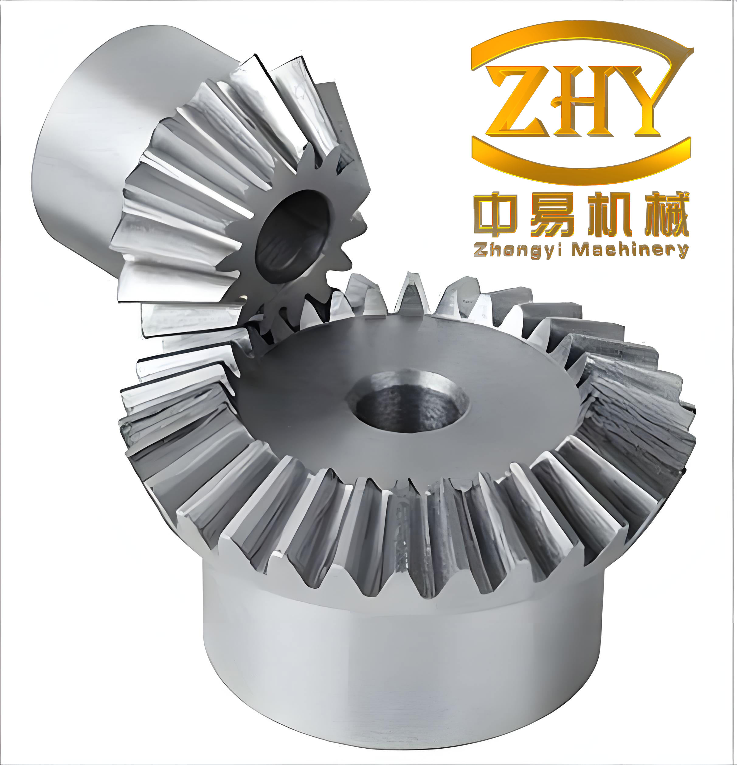
Straight bevel gears are critical components in automotive differentials, machine tools, and various mechanical power transmission systems. Their advantages include constant speed ratio, smooth transmission, and easy installation. However, during meshing, the sudden engagement of teeth in the longitudinal direction causes impact loads, leading to vibration and noise. This adversely affects the working stability and efficiency of the gear system. Therefore, investigating the dynamic performance of straight bevel gears in differentials is of great significance for reducing vehicle vibration and improving gear system performance.
Several methods exist to reduce vibration and noise in straight bevel gears, including improving manufacturing precision, changing gear structure, applying coatings, and modifying tooth profiles. Among these, tooth profile modification is considered a cost-effective and practical approach. By removing a small amount of material from specific regions of the tooth flank, it is possible to compensate for elastic deformations, manufacturing errors, and misalignments, thereby improving the contact pattern and reducing transmission errors. Although extensive research has been conducted on cylindrical gear modification, studies on straight bevel gear modification remain limited, particularly regarding the influence of modification parameters on dynamic performance.
Our research group has previously proposed modification methods such as longitudinal equidistant modification and circular arc profile modification. This paper systematically studies the dynamic performance of straight bevel gears before and after modification using advanced simulation tools. The main objectives are to:
- Develop accurate three-dimensional models of straight bevel gears using spherical involute theory.
- Establish a multi-degree-of-freedom dynamic model considering nonlinear factors.
- Simulate the dynamic behavior of unmodified and modified straight bevel gears using Romaxdesigner.
- Compare the effectiveness of different modification strategies.
- Provide guidelines for optimal modification design of straight bevel gears.
2. Three-Dimensional Solid Modeling of Straight Bevel Gears
2.1 Spherical Involute Formation
The tooth profile of straight bevel gears is a spherical involute, which is more complex than the plane involute used for cylindrical gears. The formation principle is shown in the following description: when a plane tangent to the base cone rolls purely over the base cone, the trajectory of a line on the plane generates a conical involute surface. If a sphere centered at the cone apex intersects this surface, the resulting curve is a spherical involute. The equation for the spherical involute can be expressed in Cartesian coordinates as:
$$
\begin{cases}
x = l \sin \phi \cos \theta \cos \varphi – l \sin \theta \sin \varphi \\
y = l \sin \phi \sin \theta \cos \varphi + l \cos \theta \sin \varphi \\
z = l \cos \phi \cos \varphi
\end{cases}
$$
where \( l = \sqrt{x^2 + y^2 + z^2} \) is the radius of the spherical involute starting point, \( \theta \) is the base cone angle, \( \phi \) is the angle between the generating line and the rolling plane starting line, and \( \varphi \) ranges from 0 to \( \pi/3 \). This parametric equation allows precise generation of the tooth flank geometry.
2.2 Modeling Procedure Using Matlab and SolidWorks
To create an accurate three-dimensional model of straight bevel gears, I combined Matlab with SolidWorks. The process is as follows:
- Using Matlab, I solved the spherical involute coordinates for a range of \( \varphi \) values and exported the data.
- In SolidWorks, I used the “Curve through XYZ Points” function to generate the spherical involute curves for both the large and small ends of the tooth.
- I connected the endpoints to the origin, created filled surfaces, and generated the addendum cone and dedendum cone surfaces by revolving the gear blank profile.
- I constructed ruled surfaces tangent to the two spherical involutes, trimmed the excess surfaces, and obtained the solid tooth model.
- I arrayed the tooth entities around the gear blank and cut the material to form the final gear body.
- For the pinion (planetary gear) and the side gear, I repeated the process and then assembled them with proper alignment conditions: their axes perpendicular, apices coincident, and reference planes aligned.
- I performed an interference check to ensure no geometric conflict existed in the assembly.
The parameters of the straight bevel gear pair studied in this work are listed in Table 1.
| Parameter | Side Gear | Planet Gear |
|---|---|---|
| Number of teeth | 15 | 10 |
| Cone distance (mm) | 40 | |
| Module (mm) | 4.438 | |
| Addendum height (mm) | 3.28 | 4.98 |
| Whole tooth height (mm) | 9.169 | 9.17 |
| Pressure angle (°) | 22.5 | |
| Pitch diameter (mm) | 66.57 | 44.38 |
| Pitch cone angle (°) | 56.31 | 33.69 |
| Face cone angle (°) | 66 | 46 |
| Root cone angle (°) | 44 | 24 |
This modeling method ensures high precision, avoiding the errors introduced by approximate methods such as back-cone involute generation. The resulting solid model is suitable for subsequent dynamic simulation and finite element analysis.
3. Determination of Modification Parameters
3.1 Modification Amount
The modification amount is critical for the success of tooth profile modification. If the amount is too large, the tooth strength is reduced; if too small, the modification effect is insufficient. The amount can be determined from the elastic deformation of the tooth under load. Using finite element analysis, I calculated the deformation at the large end of the pinion and side gear as 21 μm and 35 μm, respectively, when the angular velocity of the driving gear is 157 rad/s. Based on these values and considering manufacturing errors (typically 5–10 μm), I selected a modification amount of 30 μm for the longitudinal equidistant modification.
For reference, the ISO standard recommends a modification amount in the range of 10–40 μm for low-precision gears and 10–25 μm for high-precision gears. The equivalent misalignment \( F_{\beta x} \) can be used to calculate the modification amount as:
$$
\Delta \approx 0.5 F_{\beta x}
$$
Another empirical formula from Taylor Brown suggests:
$$
\Delta = 0.7 \times 10^{-3} F_m b
$$
where \( F_m \) is the normal tooth load and \( b \) is the face width.
3.2 Modification Length and Curve
The modification length is determined by the contact ratio, tooth deformation, and manufacturing errors. For straight bevel gears, I used short modification (i.e., tip relief) with the lengths listed in Table 2.
| Small end (mm) | Large end (mm) | |
|---|---|---|
| Planet gear | 1.79 | 3.0 |
| Side gear | 2.4 | 3.0 |
For the modification curve, I chose a circular arc profile, which provides a smooth transition with the involute profile, avoiding the sharp corner that would result from a straight-line modification. The continuous curvature change is beneficial for reducing dynamic excitation.
For the longitudinal direction, the effective contact area was determined according to the standard GB/T 11365-1989. For precision grades 8–9, the contact area should be 35–65% along the tooth length and 40–70% along the tooth height. This guides the extent of longitudinal modification.
4. Multi-Degree-of-Freedom Dynamic Model of Straight Bevel Gears
4.1 Dynamic Model Development
To analyze the vibration characteristics of straight bevel gears, I established a multi-degree-of-freedom lumped parameter model. The gear pair is assumed to be rigid bodies connected by a time-varying mesh stiffness and a mesh damping. The supports are considered rigid, which allows focusing on the torsional and axial vibrations of the gears. The coordinate system is defined with the origin at the intersection of the gear axes, which are perpendicular to each other (shaft angle 90°). The model includes six degrees of freedom per gear: three translational displacements along X, Y, Z axes and one torsional rotation about the gear axis. The dynamic mesh force is resolved into components along the three axes.
The relative displacement along the line of action, \( \lambda_n \), can be expressed as:
$$
\lambda_n = (X_p – X_g) c_1 + (Y_p – Y_g) c_2 + (Z_p – Z_g) c_3 + r_p \theta_p – r_g \theta_g – e_n(t)
$$
where \( c_1 = \sin \delta_p \cos \alpha_n \), \( c_2 = \cos \delta_p \cos \alpha_n \), \( c_3 = \cos \alpha_n \), \( \delta_p \) is the pitch cone angle of the pinion, \( \alpha_n \) is the normal pressure angle, \( r_p \) and \( r_g \) are the pitch radii, and \( e_n(t) \) is the static transmission error.
The dynamic mesh force \( F_n \) is given by:
$$
F_n = k_b(t) f(\lambda_n) + c_b \dot{\lambda}_n
$$
where \( k_b(t) \) is the time-varying mesh stiffness, \( c_b \) is the mesh damping, and \( f(\lambda_n) \) is a piecewise linear function representing backlash.
4.2 Governing Differential Equations
According to Newton’s second law, the equations of motion for the two gears can be written as:
$$
\begin{cases}
m_p \ddot{X}_p + c_{px} \dot{X}_p + k_{px} X_p = -F_x \\
m_p \ddot{Y}_p + c_{py} \dot{Y}_p + k_{py} Y_p = -F_y \\
m_p \ddot{Z}_p + c_{pz} \dot{Z}_p + k_{pz} Z_p = -F_z \\
I_p \ddot{\theta}_p = T_p – F_n r_p \\
m_g \ddot{X}_g + c_{gx} \dot{X}_g + k_{gx} X_g = F_x \\
m_g \ddot{Y}_g + c_{gy} \dot{Y}_g + k_{gy} Y_g = F_y \\
m_g \ddot{Z}_g + c_{gz} \dot{Z}_g + k_{gz} Z_g = F_z \\
I_g \ddot{\theta}_g = -T_g + F_n r_g
\end{cases}
$$
where \( m_p \), \( m_g \) are masses; \( I_p \), \( I_g \) are moments of inertia; \( c \) and \( k \) with subscripts denote damping and stiffness coefficients in the corresponding directions; \( T_p \) and \( T_g \) are the driving and resisting torques.
To simplify numerical solution, I introduced dimensionless variables. Let \( b_m \) be the backlash magnitude, and define dimensionless displacements as \( x_j = X_j / b_m \), \( y_j = Y_j / b_m \), \( z_j = Z_j / b_m \), \( \lambda = \lambda_n / b_m \). The dimensionless time is \( \tau = \omega_n t \), where \( \omega_n = \sqrt{k_m / m_e} \) is the natural frequency. After non-dimensionalization, the equations become:
$$
\begin{cases}
\ddot{x}_p + 2 \zeta_{px} \dot{x}_p + \kappa_{px} x_p = -f_x \\
\ddot{y}_p + 2 \zeta_{py} \dot{y}_p + \kappa_{py} y_p = -f_y \\
\ddot{z}_p + 2 \zeta_{pz} \dot{z}_p + \kappa_{pz} z_p = -f_z \\
\ddot{\theta}_p = T_p’ – F_n’ r_p’ \\
\ddot{x}_g + 2 \zeta_{gx} \dot{x}_g + \kappa_{gx} x_g = f_x \\
\ddot{y}_g + 2 \zeta_{gy} \dot{y}_g + \kappa_{gy} y_g = f_y \\
\ddot{z}_g + 2 \zeta_{gz} \dot{z}_g + \kappa_{gz} z_g = f_z \\
\ddot{\theta}_g = -T_g’ + F_n’ r_g’
\end{cases}
$$
These equations are coupled through the nonlinear mesh force \( f_n = \kappa_b(\tau) f(\lambda) + 2 \zeta_b \dot{\lambda} \).
4.3 Determination of Nonlinear Factors
Time-varying mesh stiffness is one of the most important excitations in gear dynamics. For a straight bevel gear pair, the number of tooth pairs in contact changes periodically, causing the stiffness variation. The mesh stiffness \( k_b(t) \) can be calculated by:
$$
k_b(t) = \sum_{i=1}^{n} \frac{F_i}{\delta_{1i} + \delta_{2i}}
$$
where \( F_i \) is the contact force of the \( i \)-th pair, \( \delta_{1i} \) and \( \delta_{2i} \) are the deformations of the pinion and gear teeth, and \( n \) is the number of simultaneous meshing pairs. In practice, the stiffness variation is relatively smooth for straight bevel gears, so a linearized approach can be applied.
Mesh damping can be estimated using the empirical formula proposed by Kasuba and Wang:
$$
c_b = 2 \zeta_g \sqrt{ \frac{k_m I_1 I_2}{I_1 r_2^2 + I_2 r_1^2} }
$$
where \( \zeta_g \) is the mesh damping ratio, typically in the range of 0.03–0.17, and \( r_1 \), \( r_2 \) are the pitch circle radii.
Backlash is another nonlinear factor. The piecewise function \( f(\lambda) \) is defined as:
$$
f(\lambda) =
\begin{cases}
\lambda – b_m & \lambda > b_m \\
0 & -b_m \le \lambda \le b_m \\
\lambda + b_m & \lambda < -b_m
\end{cases}
$$
Using Matlab curve fitting, I approximated this function with a cubic polynomial. The fitted expression is:
$$
f(\lambda) = a_1 \lambda + a_3 \lambda^3
$$
where \( a_1 = 0.344 \) and \( a_3 = 1.201 \times 10^7 \) for \( b_m = 5 \times 10^{-5} \) m. The polynomial provides sufficient accuracy for solving the dynamic equations.
4.4 Solution Method
The governing equations are nonlinear ordinary differential equations. I applied the Adomian decomposition method to obtain semi-analytical solutions. Introducing state variables \( u_1 = x_p \), \( u_2 = \dot{x}_p \), …, the equations are transformed into a state-space form:
$$
\dot{\mathbf{u}} = \mathbf{H} \mathbf{u} + \mathbf{N}(\mathbf{u}) + \mathbf{G}(\tau)
$$
where \( \mathbf{H} \) is the linear matrix, \( \mathbf{N} \) contains nonlinear terms, and \( \mathbf{G} \) is the excitation vector. The solution is expressed as:
$$
\mathbf{u}(\tau) = \sum_{j=0}^{\infty} \mathbf{u}_j(\tau)
$$
with each \( \mathbf{u}_j \) computed recursively via the Adomian polynomials. This method yields the displacement and velocity responses. For the tooth backlash function, the Adomian polynomials take simple forms depending on the sign of the relative displacement. The series converges quickly, and retaining five to six terms is usually sufficient for engineering accuracy.
5. Dynamic Simulation Using Romaxdesigner
5.1 Simulation Setup
Romaxdesigner is a specialized software for transmission system analysis, offering static and dynamic analysis, NVH analysis, and optimization. The workflow is:
- Import the solid model of the straight bevel gear pair (in STL format from SolidWorks) into Romaxdesigner.
- Define the material properties, support bearings, shafts, and load cases.
- Set the input speed and torque: I used an input speed of 1500 r/min and a torque of 100 N·m, representing an automotive driving condition with a duration of 5 hours.
- Run static analysis to obtain gear strength, safety factors, and bearing loads.
- Perform transmission error analysis and NVH analysis to obtain dynamic responses.
Static analysis confirmed that both gears pass the strength criteria. Table 3 shows the safety factors, and Table 4 lists the gear life predictions.
| Gear | Contact stress (MPa) | Bending stress (MPa) | Safety factor (contact) | Safety factor (bending) |
|---|---|---|---|---|
| Side gear | 2385.65 | 521.05 | 1.025 | 1.208 |
| Planet gear | 2385.65 | 274.87 | 1.000 | 2.181 |
| Gear | Contact life (hrs) | Bending life (hrs) | Combined life (hrs) | Result |
|---|---|---|---|---|
| Side gear | 7.50 | 24.36 | 7.50 | Pass |
| Planet gear | 5.00 | 1.085e15 | 5.00 | Pass |
These results indicate that the gear system can operate safely under the specified load case, which is a prerequisite for dynamic analysis.
5.2 Transmission Error Analysis
Transmission error is one of the main internal excitations in gear systems. It is defined as the difference between the actual and ideal angular positions of the driven gear, expressed as a linear displacement along the line of action. In Romaxdesigner, I computed the dynamic transmission error (DTE) for the unmodified and modified gear pairs. The results are presented in Figures 1 to 3 (not shown but described here).
For the unmodified straight bevel gear pair, the maximum dynamic transmission error reached 3.39 μm, with a peak-to-peak value of 0.87 μm. The dynamic contact load peaked at 521 N. The frequency range from 400 to 1120 Hz corresponds to an input speed range of 1080–3300 r/min, where the transmission error and contact load exhibited significant fluctuations, indicating high vibration and noise.
After performing longitudinal equidistant modification, the maximum transmission error dropped to 1.13 μm, a reduction of about 67%. The peak-to-peak value decreased to 0.29 μm, and the maximum dynamic contact load reduced to 170.2 N. Similarly, after circular arc profile modification, the maximum transmission error was 1.19 μm (a 65% reduction), with a peak-to-peak of 0.41 μm and a maximum dynamic contact load of 173.6 N. The frequency response also showed much lower amplitudes in the range of 400–1120 Hz.
5.3 Natural Frequency and Modal Analysis
Understanding the natural frequencies of the gear system helps identify potential resonance conditions. Romaxdesigner computed the first ten natural frequencies of the straight bevel gear pair, as listed in Table 5.
| Order | 1 | 2 | 3 | 4 | 5 | 6 | 7 | 8 | 9 | 10 |
|---|---|---|---|---|---|---|---|---|---|---|
| Frequency (Hz) | 109.96 | 1893.2 | 2089.3 | 2362.5 | 2634.1 | 2673.7 | 3342.8 | 4022.7 | 4126.9 | 4529.6 |
For the given operating condition, the mesh frequency is \( f_m = 10 \times 157 / (2\pi) = 249.87 \) Hz. None of the natural frequencies coincide with this mesh frequency or its harmonics, so resonance is not expected under steady-state conditions. However, when the input speed varies, the mesh frequency could pass through some critical speeds, which should be avoided by design.
5.4 Vibration Response (NVH)
To evaluate the dynamic response, I used the dynamic transmission error as the excitation and computed the linear modal compliance (displacement per unit force) of the gear pair. The frequency response function indicates the vibration sensitivity across the frequency spectrum.
For the unmodified gear set, the maximum modal compliance occurred at 730 Hz with a value of \( 4.96 \times 10^{-4} \) μm/N. This frequency contributes the most to the overall vibration and noise. After longitudinal equidistant modification, the maximum modal compliance reduced to \( 1.01 \times 10^{-4} \) μm/N at the same frequency (730 Hz), which is a 79.6% reduction. After circular arc profile modification, the maximum value was \( 1.35 \times 10^{-4} \) μm/N, but it occurred at a different frequency (1830 Hz). These results clearly indicate that modification effectively suppresses the vibration amplitudes.
5.5 Comparison of Dynamic Performance
I summarized the key dynamic performance indicators in Table 6.
| Indicator | Unmodified | Circular arc modification | Longitudinal equidistant modification |
|---|---|---|---|
| Maximum dynamic transmission error (μm) | 3.39 | 1.19 | 1.13 |
| Maximum dynamic contact load (N) | 521 | 173.6 | 170.2 |
| Maximum linear modal compliance (μm/N) | \(4.96 \times 10^{-4}\) | \(1.35 \times 10^{-4}\) | \(1.01 \times 10^{-4}\) |
| Reduction in transmission error | — | 65% | 67% |
| Reduction in vibration amplitude | — | 73% | 79% |
Both modification methods significantly improve the dynamic behavior of straight bevel gears. The longitudinal equidistant modification outperforms the circular arc profile modification in reducing transmission error, dynamic load, and vibration amplitude. This is because the longitudinal equidistant modification more effectively compensates for the non-uniform load distribution along the tooth width, thereby reducing the excitation caused by edge contact and stress concentration.
6. Discussion on Dynamic Excitations and Performance Indicators
6.1 Dynamic Excitation Sources
The dynamic response of a gear system is influenced by both internal and external excitations. Internal excitations include:
- Stiffness excitation: caused by the periodic variation of mesh stiffness as the number of contacting tooth pairs changes.
- Error excitation: due to manufacturing and assembly errors, which produce transmission error.
- Mesh impact excitation: arising from the sudden engagement and disengagement of teeth, especially when the base pitch of the mating gears differs.
External excitations come from the prime mover’s torque fluctuations and the driven load’s variations. In my simulation, I considered the torque and speed as constant, focusing on the internal excitations that dominate under steady-state operating conditions.
6.2 Performance Indicators
Several indicators are used to evaluate the dynamic performance of straight bevel gears:
Dynamic load factor \( K_v \): the ratio of the maximum dynamic tooth load to the static load. Lower values indicate better dynamic performance.
Average mesh stiffness \( \bar{k} \): computed over one mesh cycle, reflecting the overall load-carrying capability.
RMS value of stiffness fluctuation: a measure of the intensity of the stiffness variation, which directly correlates with vibration excitation.
Vibration acceleration level: measured at the bearing or housing, representing the noise and vibration severity.
In this study, I used dynamic transmission error, dynamic contact load, and linear modal compliance as the primary indicators. The results show that modification effectively reduces all these indicators, confirming that tooth profile modification is a valid technique for improving the dynamic performance of straight bevel gears.
7. Conclusion and Future Work
7.1 Conclusions
In this work, I investigated the dynamic performance of modified straight bevel gears through a combination of precise geometric modeling, dynamic mathematical modeling, and simulation using Romaxdesigner. The key conclusions are:
- Accurate three-dimensional models of straight bevel gears can be created using spherical involute equations in Matlab and SolidWorks. This method avoids the errors of approximate modeling and provides a reliable basis for dynamic simulation.
- Tooth profile modification, whether by circular arc profile or longitudinal equidistant modification, significantly reduces the dynamic transmission error and dynamic contact load of straight bevel gears. The maximum transmission error decreased by more than 65% compared with the unmodified case.
- The longitudinal equidistant modification is more effective than the circular arc profile modification in reducing vibration and noise. It reduced the maximum linear modal compliance by 79%, compared with 73% for the circular arc modification.
- The multi-degree-of-freedom dynamic model, including time-varying stiffness, damping, and backlash, is suitable for describing the nonlinear behavior of straight bevel gears. The Adomian decomposition method provides a feasible way to solve the nonlinear differential equations.
- Static analysis confirmed that the gear system meets the strength and life requirements under the specified load condition, ensuring the validity of the subsequent dynamic analysis.
7.2 Future Work
Although this study provides valuable insights, several aspects require further investigation:
- Experimental validation: I plan to conduct physical experiments on modified straight bevel gears to verify the simulation results and further refine the modification parameters.
- Thermal effects: In high-speed or heavily loaded applications, thermal deformation can significantly affect gear performance. Future research should consider the combined effect of elastic and thermal deformation on modification design.
- Nonlinear dynamic analysis: The full nonlinear dynamics, including bifurcation and chaos, should be explored to understand the stability boundaries of the system. More advanced numerical methods may be required to handle multiple nonlinearities.
- Multi-objective optimization: An optimization framework that simultaneously considers vibration, noise, and strength could help determine the best modification parameters for various working conditions.
- System-level analysis: Including the flexibility of shafts, bearings, and housing in the model would provide a more comprehensive understanding of the gear system dynamics.
In summary, this research demonstrates that proper tooth profile modification is an effective and practical approach to enhance the dynamic performance of straight bevel gears. The results offer useful guidelines for the design and manufacturing of quiet and reliable gear transmissions.