
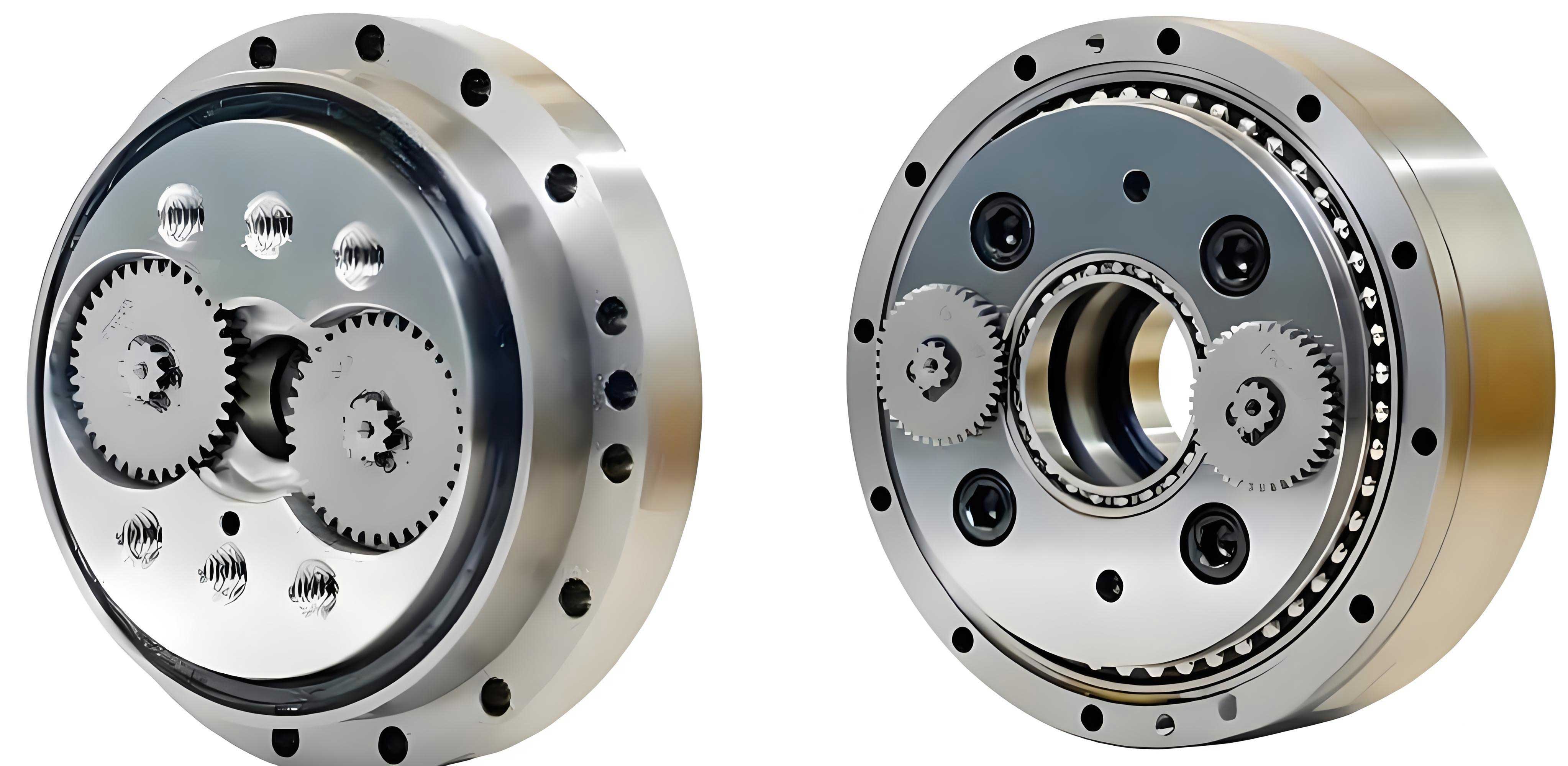
In the landscape of modern industrial robotics, the pursuit of reliability and predictive maintenance has become paramount. Among the critical components demanding meticulous attention is the rotary vector reducer, a core element in robotic elbow joints. Its complex internal structure, involving cycloidal gears and planetary mechanisms, makes it particularly susceptible to wear and failures such as pitting, surface abrasion, and even tooth breakage. These faults can lead to unplanned downtime, reduced precision, and significant economic loss. Therefore, developing robust and accurate fault diagnosis methods for the rotary vector reducer is a significant research challenge with direct implications for industrial productivity and safety. This article presents a novel diagnostic framework that combines a Continuous Hidden Markov Model (CHMM) with the Artificial Bee Colony (ABC) optimization algorithm, aiming to overcome the inherent stability limitations of traditional models and achieve superior fault classification accuracy for the rotary vector reducer.
The operational state of a rotary vector reducer is primarily reflected in its vibration signals. However, these signals are often non-stationary, noisy, and contain subtle signatures of incipient faults. Traditional diagnosis methods, including time-domain statistical analysis, frequency spectrum examination, and time-frequency techniques like wavelet transforms, have been widely applied. While effective for clear fault signatures, their performance degrades with complex signal patterns and overlapping fault features. Data-driven approaches, particularly those based on machine learning and statistical models, have shown great promise. Techniques such as Support Vector Machines (SVMs) and neural networks, including CS-BP networks combined with Ensemble Empirical Mode Decomposition (EEMD), have been explored for rotary vector reducer diagnosis. However, these models often require large labeled datasets and may struggle with the temporal dynamics and probabilistic nature of degradation processes.
This is where probabilistic graphical models like the Hidden Markov Model (HMM) offer a distinct advantage. An HMM is a doubly stochastic process that models a system as evolving through a series of unobserved (hidden) states, with each state emitting observable symbols according to a probability distribution. It is particularly suited for modeling time-series data where the underlying state sequence is not directly visible but influences the observable outputs. For continuous-valued vibration signals, the Continuous HMM (CHMM) is employed, where the observation probability in each state is modeled by a continuous probability density function, typically a Gaussian Mixture Model (GMM). This allows the CHMM to effectively capture the complex, multi-modal distribution of feature vectors extracted from vibration data of a rotary vector reducer under different health states.
The standard procedure for fault diagnosis using a CHMM involves two phases: training and classification. First, feature vectors are extracted from the vibration signals. A powerful method for this is Wavelet Packet Decomposition (WPD). WPD provides a more detailed frequency-band analysis than standard wavelet decomposition. Using a suitable mother wavelet (e.g., db3), the signal is decomposed into multiple levels, and specific nodes are selected for reconstruction. The energy of each reconstructed signal component serves as a highly informative feature. For a signal decomposed to the 3rd level, we obtain 8 frequency bands (j=0,1,…,7). The energy $E_{3j}$ of the reconstructed signal $s_{3j}(t)$ from node $j$ is calculated as:
$$E_{3j} = \int |s_{3j}(t)|^2 dt = \sum_{k=1}^{n} |x_{jk}|^2$$
where $x_{jk}$ are the wavelet coefficients. To form a consistent feature vector, these energy values are normalized:
$$o_{3j} = \frac{e_{3j} – \min(\mathbf{E_{3}})}{\max(\mathbf{E_{3}}) – \min(\mathbf{E_{3}})}$$
where $\mathbf{E_{3}} = [E_{30}, E_{31}, …, E_{37}]$ and $\mathbf{O_{3}} = [o_{30}, o_{31}, …, o_{37}]$ is the resulting normalized feature vector. A separate CHMM $\lambda = (\pi, \mathbf{A}, \mathbf{B})$ is then trained for each known fault state of the rotary vector reducer (e.g., normal, pitting, wear, broken tooth) using sequences of these feature vectors. The model parameters include the initial state distribution $\pi$, the state transition probability matrix $\mathbf{A}$, and the observation probability matrix $\mathbf{B}$, which is defined by GMM parameters (mixture weights, mean vectors, and covariance matrices). The Baum-Welch algorithm, an Expectation-Maximization (EM) procedure, is typically used for training.
During classification, a sequence of feature vectors from an unknown state of the rotary vector reducer is presented to each trained CHMM. The forward algorithm is used to compute the likelihood $P(O|\lambda_i)$ that the observation sequence $O$ was generated by model $\lambda_i$. The fault type corresponding to the model yielding the highest likelihood is assigned as the diagnosis.
Despite its strengths, the classical CHMM trained with the Baum-Welch algorithm has a critical flaw for practical diagnosis of the rotary vector reducer: high sensitivity to initial parameters. The Baum-Welch algorithm is guaranteed only to find a local maximum of the likelihood function. Different initializations of the GMM parameters (means $\mu_{jl}$, covariances $\mathbf{U}_{jl}$, and mixture weights $c_{jl}$) can lead to significantly different trained models, resulting in inconsistent and unstable diagnostic performance. This instability is unacceptable for industrial applications where reliability is key. To stabilize and enhance the diagnostic performance for the rotary vector reducer, we propose to optimize the initial model parameters before the Baum-Welch refinement using a global optimization metaheuristic: the Artificial Bee Colony (ABC) algorithm.
The ABC algorithm is a swarm intelligence technique inspired by the foraging behavior of honey bees. It maintains a population of candidate solutions (“food sources”), each represented by a vector of parameters to be optimized. The colony consists of employed bees, onlooker bees, and scout bees, which cooperate to explore and exploit the solution space. Its advantages include strong global search capability, relatively few control parameters, and robustness. We integrate ABC into the CHMM training workflow to find a superior initial point for the Baum-Welch algorithm, thereby guiding it toward a better, more stable local optimum (ideally the global optimum) for the model representing each fault state of the rotary vector reducer.
The integration, termed ABC-CHMM, proceeds as follows for each fault class of the rotary vector reducer:
1. Solution Representation & Objective: A food source (solution) $\mathbf{x}_i$ encodes the key parameters of a CHMM that critically affect the Baum-Welch starting point: the means $\mu_{jl}$ and mixture weights $c_{jl}$ of the GMMs for all hidden states. The covariance matrices $\mathbf{U}_{jl}$ are often initialized as identity matrices or based on the global data variance. The objective is to maximize the likelihood that the initial model $\lambda(\mathbf{x}_i)$ generates the training observation sequences $O$. Since ABC is typically formulated for minimization, we define the fitness function $f(\mathbf{x}_i)$ and the fitness value $F_i$ as:
$$f(\mathbf{x}_i) = \frac{1}{P(O | \lambda(\mathbf{x}_i)) + C}, \quad F_i = \frac{1}{1 + f(\mathbf{x}_i)}$$
where $C$ is a small constant to prevent division by zero, and $P(O | \lambda(\mathbf{x}_i))$ is computed via the forward algorithm. A higher output probability corresponds to a lower $f(\mathbf{x}_i)$ and a higher fitness $F_i$.
2. ABC Optimization Phase:
- Employed Bee Phase: Each employed bee associated with a food source $\mathbf{x}_i$ performs a local search in its neighborhood to find a new candidate $\mathbf{v}_i$:
$$v_{ij} = x_{ij} + \phi_{ij}(x_{ij} – x_{kj})$$
where $k$ is a randomly chosen index different from $i$, and $\phi_{ij}$ is a random number in $[-1, 1]$. A greedy selection is applied between $\mathbf{x}_i$ and $\mathbf{v}_i$ based on their fitness. - Onlooker Bee Phase: Onlooker bees select food sources probabilistically based on their fitness using a roulette wheel selection: $p_i = F_i / \sum_{n=1}^{SN} F_n$. They then perform the same local search and greedy selection on the chosen sources, intensifying the search around high-quality solutions.
- Scout Bee Phase: If a food source’s fitness cannot be improved after a predetermined number of trials (“limit”), it is abandoned. The employed bee for that source becomes a scout bee and discovers a new random food source:
$$x_{ij} = x_{\min, j} + \text{rand}(0,1) \cdot (x_{\max, j} – x_{\min, j})$$
This mechanism ensures exploration and avoids premature convergence.
3. CHMM Refinement Phase: Once the ABC algorithm terminates (after a maximum number of cycles), the best-found solution $\mathbf{x}_{\text{best}}$ is decoded into an initial CHMM $\lambda_{\text{init}}$. This model is then fed into the standard Baum-Welch algorithm for final, precise parameter estimation using the same training data. The refined model $\lambda_{\text{final}}$ is saved as the representative model for that specific fault state of the rotary vector reducer.
This hybrid approach leverages the global exploration strength of ABC to find a promising region in the complex parameter space, followed by the local exploitation power of Baum-Welch to fine-tune the model. The process effectively “de-sensitizes” the final model to the randomness of initialization, leading to markedly improved diagnostic stability for the rotary vector reducer.
To validate the proposed ABC-CHMM method for the rotary vector reducer, a series of experiments were conducted on a mechanical fault simulation platform (QPZZ-II). Vibration signals were collected from a rotary vector reducer under four distinct conditions: Normal, Tooth Pitting, Surface Wear, and Broken Tooth. The sampling frequency was set at 5105 Hz. Key gear parameters for the test setup are summarized below.
| Gear | Module | Number of Teeth | Material |
|---|---|---|---|
| Large Gear | 2 | 75 | S45C |
| Small Gear | 2 | 55 | S45C |
The raw vibration waveforms for the four states show visible differences, but definitive classification from the time-domain alone is challenging. Feature extraction via 3-level db3 WPD was performed. The normalized energy distribution across the 8 frequency bands provides a much clearer signature, as conceptually shown in the analysis of the energy patterns which revealed that specific faults in the rotary vector reducer cause distinct energy mutations in particular frequency bands. For instance, one specific frequency node exhibited very low energy for both Normal and Pitting states, but very high energy for Wear and Broken Tooth states, providing a strong discriminative feature.
Multiple models were trained and compared: a standard CHMM with random initialization (CHMM-Random) and the proposed ABC-optimized CHMM (ABC-CHMM). The ABC algorithm successfully converged, optimizing the initial model parameters. The training process itself demonstrated the efficiency of the proposed method. While the standard CHMM required 26 iterations of Baum-Welch (taking approximately 93.58 seconds) to converge, the ABC-CHMM, starting from a superior initial point, converged in only 16 iterations (taking about 38.73 seconds), representing a significant reduction in training time for the rotary vector reducer diagnostic model.
The core diagnostic performance is evaluated by the model’s output probability (log-likelihood) for test sequences. A well-trained model should assign the highest log-likelihood to test sequences from its own fault class. The analysis of logarithmic output probabilities for test samples revealed a critical weakness in the standard CHMM. Due to suboptimal training from poor initialization, the differences in output probability between the correct and some incorrect models for certain test samples were minuscule (less than $2.6 \times 10^{-11}$), making reliable classification impossible. Quantitatively, there were 7 such ambiguous/erroneous classification points across the test set when using the standard CHMM.
| Diagnosis Model | Training Time (s) | Iterations to Converge | Ambiguous Test Samples | Average Accuracy |
|---|---|---|---|---|
| Standard CHMM | 93.58 | 26 | 7 | ~87.6% |
| ABC-Optimized CHMM | 38.73 | 16 | 0 | ~99% |
The performance of the ABC-CHMM model was strikingly different. The optimization led to models that produced output probabilities with much clearer separation. For every test sequence from the rotary vector reducer, the correct model yielded a significantly higher log-likelihood than all other models, eliminating classification ambiguity. The quantitative result was a dramatic leap in diagnostic accuracy. The standard CHMM achieved an accuracy of approximately 87.6%, primarily hampered by the 7 ambiguous samples. In contrast, the proposed ABC-CHMM method boosted the average fault diagnosis accuracy for the rotary vector reducer to nearly 99%.
This investigation successfully developed and validated a hybrid ABC-CHMM fault diagnosis framework specifically for the rotary vector reducer. The method directly addresses the critical instability issue in standard CHMM training caused by parameter initialization sensitivity. By employing the Artificial Bee Colony algorithm as an intelligent global search mechanism to find superior initial model parameters, the subsequent Baum-Welch algorithm is consistently guided toward a more optimal and stable solution. The results are compelling: the ABC-CHMM model not only converges faster during training but also achieves a decisive improvement in classification performance, elevating accuracy from approximately 87.6% to nearly 99%. This level of reliability is essential for practical industrial deployment. The proposed method, therefore, offers a powerful, stable, and efficient tool for the condition monitoring and predictive maintenance of rotary vector reducers, with potential applicability to a wide range of other complex rotating machinery and transmission systems where vibration-based fault diagnosis is employed.