
In my research, I focus on developing a precise and efficient method for modeling spiral bevel gears by directly simulating the actual gear cutting process. Traditional manufacturing of these gears, which are critical components in automotive, aerospace, and industrial machinery due to their high load capacity and smooth transmission, often relies on trial-and-error adjustments using Gleason machine settings. This approach is time-consuming and heavily dependent on operator skill. To overcome these limitations, I propose a virtual gear cutting methodology that replicates the physical cutting actions, enabling accurate digital twin creation, parameter optimization, and dynamic interference detection before any physical prototype is made. This article details my comprehensive framework, encompassing mathematical derivation, software implementation, 3D CAD modeling, and simulation validation, all centered around the actual gear cutting mechanics.
The core innovation lies in mimicking the exact gear cutting sequence where the tooth flank is generated as an envelope of successive cutter blade positions. Unlike theoretical conjugate surface approaches, my method treats the tooth surface as a collection of points derived from the intersections of adjacent cutter traces during the continuous gear cutting motion. By reducing the time interval between cuts to an infinitesimally small value, the error between the simulated flank and the ideal envelope can be minimized to an acceptable tolerance. This gear cutting simulation forms the basis for all subsequent steps.
To mathematically describe this process, I established a series of coordinate systems corresponding to the Gleason-type gear cutting machine. Let $S_0$ be the fixed machine coordinate system with its origin at the machine center. The cutter head and worktable motions are represented by dynamic coordinate systems: $S_1$ (attached to the cradle), $S_2$ (cutter spindle), $S_3$ (cutter tilt body), and $S_4$ (cutter blade itself). The workpiece coordinate system $S_{1′}$ is defined relative to $S_0$ through translations and rotations involving machine settings like vertical offset $E$, axial offset $X$, and bed distance $X_B$. The transformation matrix from the cutter coordinate system $S_4$ to the workpiece system $S_{1′}$ at any time $t$ is denoted as $\mathbf{M}_{41′}(t)$, which incorporates cradle rotation angle $q$, cutter rotation angle $\theta$, cutter tilt angle $i$, and workpiece rotation angle $\phi$.
Consider a straight blade cutter with pressure angle $\alpha$ and tip radius $r_a$. At time $t$, the cutting edge line in $S_4$ for one blade is given by:
$$ \begin{align*}
X_4 &= r_a u + r_a, \\
Y_4 &= 0, \\
Z_4 &= -r_a u \cot \alpha,
\end{align*} $$
where $u$ is a parameter. Transforming this line to $S_{1′}$ using $\mathbf{M}_{41′}(t)$ yields the trace line on the workpiece at time $t$. After a small time increment $\Delta t$, the workpiece rotates by $\omega_1 \Delta t$, the cradle by $\omega_2 \Delta t$, and the cutter by $\omega_3 \Delta t$. The trace from the first blade at time $t$ evolves due to workpiece rotation, while a subsequent blade (e.g., the next blade on the cutter head, separated by an angle $2\pi/n$ where $n$ is the number of blades) begins cutting at time $t+\Delta t$. Its edge line in $S_4$ is:
$$ \begin{align*}
X_4 &= r_a \cos(2\pi/n) u + r_a \cos(2\pi/n), \\
Y_4 &= r_a \sin(2\pi/n) u + r_a \sin(2\pi/n), \\
Z_4 &= -r_a \sin(2\pi/n) u \cot \alpha.
\end{align*} $$
Transforming this second line to $S_{1′}$ at time $t+\Delta t$ using the updated matrix $\mathbf{M}_{41′}(t+\Delta t)$ gives a new trace. The tooth flank point is approximated as the intersection point of these two adjacent trace lines in $S_{1′}$. If the lines are skew, I use the midpoint of their common perpendicular segment. The coordinates $(X_{1′}, Y_{1′}, Z_{1′})$ of this point are derived by solving the line equations. For the case of intersection, the point is given by:
$$ \begin{align*}
X_p &= A – a \left( \frac{(A – A’)c’ + a'(C’ – C)}{a c’ – a’ c} \right), \\
Y_p &= B – b \left( \frac{(A – A’)c’ + a'(C’ – C)}{a c’ – a’ c} \right), \\
Z_p &= C + c \left( \frac{(A – A’)c’ + a'(C’ – C)}{a c’ – a’ c} \right),
\end{align*} $$
where $A, B, C$ are constants from the first line equation, $a, b, c$ are its direction cosines, $A’, B’, C’$ and $a’, b’, c’$ are corresponding terms for the second line, all functions of machine settings and time. By iterating this over multiple blades and time steps, I generate a dense point cloud representing the entire tooth surface, directly linked to the gear cutting parameters.
The relationship between machine settings and the resulting gear geometry is complex. To facilitate analysis, I summarize key gear cutting parameters and their effects in the following table:
| Gear Cutting Parameter | Symbol | Influence on Tooth Flank |
|---|---|---|
| Radial Tool Distance | $S_r$ | Controls tooth depth and profile curvature |
| Angular Tool Position | $q$ | Affects spiral angle and contact pattern |
| Cutter Tilt Angle | $i$ | Modifies pressure angle along face width |
| Machine Center to Back (Bed) | $X_B$ | Adjusts tooth taper and root line |
| Workpiece Offset (Vertical) | $E$ | Influences bias and surface mismatch |
| Velocity Ratio (Roll) | $R_v$ | Determines lengthwise crowning and conjugation |
Implementing this mathematical model requires robust computation. I developed a dedicated gear cutting simulation program using Visual Basic (VB), which automates the calculation and adjustment of all machine settings. The program flow is as follows: input basic gear design parameters (number of teeth, module, spiral angle, pressure angle, etc.); compute derived geometric parameters; then iteratively adjust gear cutting settings like cutter radius, tool positions, and machine offsets while generating tooth flank points. The user interface consists of four dialog boxes: Initial Parameter Input, Basic Parameter Calculation, Pinion Gear Cutting Adjustment, and Gear Gear Cutting Adjustment. This allows interactive tuning of the gear cutting process to achieve desired tooth contact characteristics.
To illustrate, consider a gear pair with parameters used in my case study:
| Parameter | Pinion | Gear |
|---|---|---|
| Number of Teeth | 11 | 25 |
| Module (mm) | 9 | |
| Pressure Angle (°) | 20 | |
| Spiral Angle (°) | 35 | |
| Shaft Angle (°) | 90 | |
| Face Width (mm) | 41 | |
| Hand of Spiral | Left | Right |
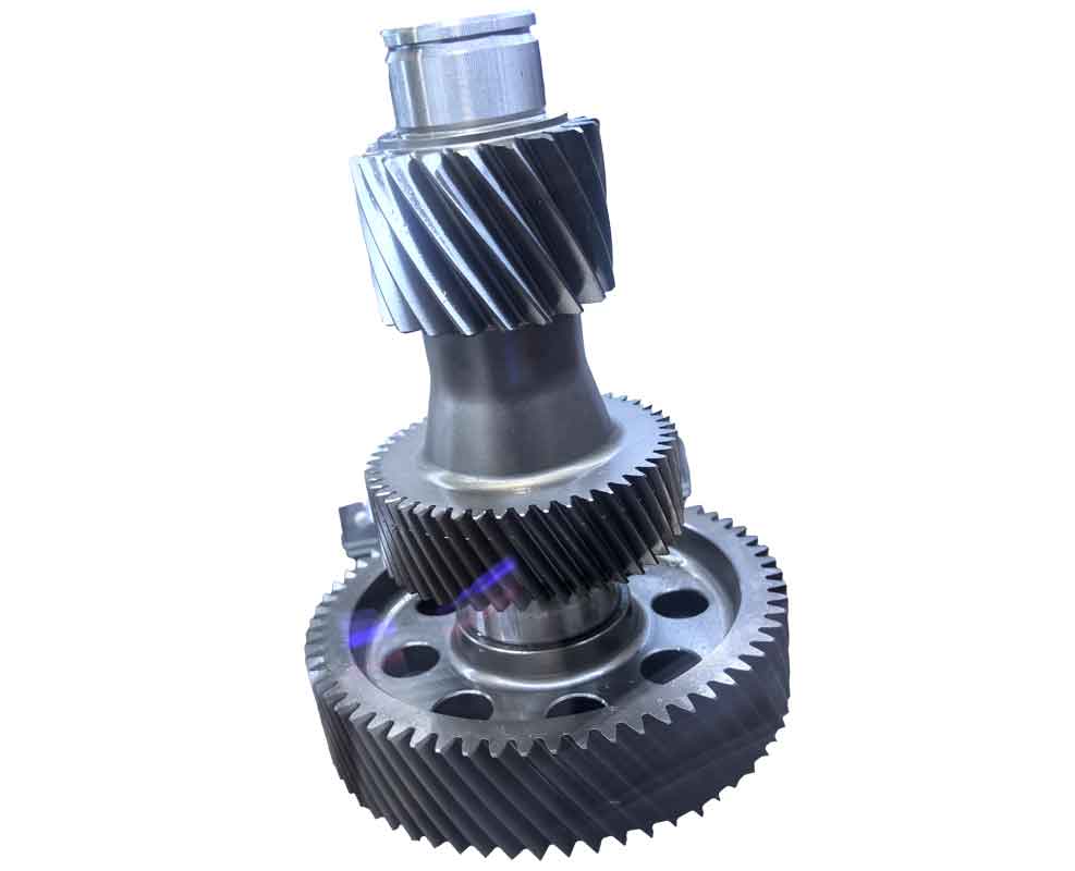
After running the gear cutting program with initial settings, I obtain a data file containing thousands of $(X, Y, Z)$ points for each tooth flank. These points serve as the foundation for 3D CAD model construction. I use Pro/ENGINEER (Pro/E) for this purpose, following a structured modeling workflow. First, the point cloud is imported and processed to create spline curves representing tooth profiles at various sections along the face width. These curves are used as骨架 lines. Next, using boundary blend functions, I generate the convex and concave flank surfaces for a single tooth slot. The root surface is created by connecting the bottom edges of the flanks, and all surfaces are merged into a single quilt. Finally, this quilt is solidified to cut the tooth slot from a blank gear model. The slot is then patterned circumferentially to complete the full gear. For visualization, here is an example of a modeled spiral bevel gear generated through this gear cutting-based approach:
The gear cutting simulation does not end with single gear modeling. A critical phase is the virtual assembly and dynamic interference detection of the gear pair. In Pro/E, I assemble the pinion and gear according to their theoretical shaft angle and offset. Then, I perform a motion analysis where the gears are rotated through multiple mesh cycles. The interference detection tool checks for collisions or undesired contact between tooth surfaces at every incremental position. This dynamic simulation reveals the quality of the mesh, including the contact pattern and potential edge loading. If interference or poor contact is detected, I return to the gear cutting program, adjust parameters (e.g., modify cutter offset or machine roll ratio), regenerate the flank points, and update the CAD models. This iterative loop—gear cutting parameter adjustment, point generation, 3D modeling, and dynamic testing—constitutes a virtual try-out that mirrors physical试切 but is far faster and more cost-effective.
The mathematical framework can be extended to sensitivity analysis. Let $\mathbf{P}$ be a vector of gear cutting parameters (e.g., $\mathbf{P} = [S_r, q, i, X_B, E, R_v]^T$), and let $\mathbf{F}(u, v, \mathbf{P})$ represent the tooth surface point as a function of surface parameters $u, v$ and $\mathbf{P}$. The sensitivity of the surface to a parameter change is given by the Jacobian:
$$ \mathbf{J} = \frac{\partial \mathbf{F}}{\partial \mathbf{P}} = \begin{bmatrix}
\frac{\partial X}{\partial S_r} & \frac{\partial X}{\partial q} & \cdots & \frac{\partial X}{\partial R_v} \\
\frac{\partial Y}{\partial S_r} & \frac{\partial Y}{\partial q} & \cdots & \frac{\partial Y}{\partial R_v} \\
\frac{\partial Z}{\partial S_r} & \frac{\partial Z}{\partial q} & \cdots & \frac{\partial Z}{\partial R_v}
\end{bmatrix}. $$
By computing these partial derivatives numerically through finite differences in the gear cutting simulation, I can quantify how each machine setting influences tooth geometry. For instance, a change in radial distance $\Delta S_r$ primarily alters the tooth depth $\Delta h$, approximately related by $\Delta h \approx \Delta S_r \cdot \sin(\alpha)$. Such relationships aid in systematic gear cutting correction.
Furthermore, the gear cutting point generation algorithm can be optimized for computational efficiency. The core operation involves solving for line intersections millions of times. I implemented a vectorized approach where multiple points are computed simultaneously. For a given time step $\Delta t$, the condition for line intersection in 3D can be expressed using the determinant of a matrix formed by direction vectors and the vector connecting points on the two lines. Let lines $L_1$ and $L_2$ be defined by points $\mathbf{p}_1, \mathbf{p}_2$ and directions $\mathbf{d}_1, \mathbf{d}_2$. They intersect if:
$$ \left| (\mathbf{p}_2 – \mathbf{p}_1) \cdot (\mathbf{d}_1 \times \mathbf{d}_2) \right| < \epsilon, $$
where $\epsilon$ is a tolerance. The intersection point $\mathbf{p}$ is found via:
$$ \mathbf{p} = \mathbf{p}_1 + s \mathbf{d}_1 = \mathbf{p}_2 + t \mathbf{d}_2, $$
$$ s = \frac{(\mathbf{p}_2 – \mathbf{p}_1) \times \mathbf{d}_2 \cdot (\mathbf{d}_1 \times \mathbf{d}_2)}{\|\mathbf{d}_1 \times \mathbf{d}_2\|^2}, \quad t = \frac{(\mathbf{p}_2 – \mathbf{p}_1) \times \mathbf{d}_1 \cdot (\mathbf{d}_1 \times \mathbf{d}_2)}{\|\mathbf{d}_1 \times \mathbf{d}_2\|^2}. $$
In my gear cutting code, I precompute transformation matrices for discrete time steps to avoid redundant calculations.
The advantages of this gear cutting-based modeling approach are manifold. First, it directly ties the digital model to manufacturable machine settings, ensuring that the designed gear can be physically produced. Second, it enables comprehensive virtual testing, reducing reliance on costly physical prototypes. Third, it allows for rapid exploration of design alternatives by tweaking gear cutting parameters and immediately observing their effects on tooth contact and strength. To quantify these benefits, I conducted a comparative study between traditional trial-and-error gear cutting and my virtual method:
| Aspect | Traditional Physical Gear Cutting | Virtual Gear Cutting Simulation |
|---|---|---|
| Time per Iteration | Hours to days (setup, cutting, inspection) | Minutes (computation and CAD update) |
| Material Cost | High (waste from试切 blanks) | Negligible (digital only) |
| Parameter Adjustment Flexibility | Limited by machine physical limits | Highly flexible, broad parameter ranges |
| Contact Pattern Prediction | Requires staining compounds and testing | Direct visualization via interference detection |
| Skill Dependency | High (experienced operator needed) | Reduced (automated algorithms) |
My method also integrates with finite element analysis (FEA) for stress evaluation. After obtaining the 3D model from gear cutting simulation, I export it to FEA software to perform loaded tooth contact analysis. The accurate geometry ensures reliable stress predictions. The contact pattern under load can be compared with the unloaded interference results to further refine gear cutting parameters for optimal performance.
In conclusion, I have developed a holistic digital workflow for spiral bevel gears rooted in the actual gear cutting process. By simulating the cutter-workpiece engagement kinematics, I derive a mathematical model that generates precise tooth flank points. These points are used to build faithful 3D CAD models, which undergo dynamic assembly and interference checks to validate mesh quality. The entire process is driven by adjustable gear cutting parameters, enabling virtual try-out and optimization without material waste. This approach significantly shortens development cycles, lowers costs, and enhances gear quality by providing a direct link between design intent and manufacturing reality. Future work will focus on extending the gear cutting simulation to more complex cutter profiles, such as those with modified edges for finishing, and integrating real-time optimization algorithms to automatically determine the best gear cutting settings for given performance criteria.
The gear cutting methodology I present is not limited to spiral bevel gears; it can be adapted to other gear types generated by continuous cutting processes, such as hypoid gears or face gears. The core principle remains: emulate the physical cutting tool path to create a digital twin. As manufacturing moves towards Industry 4.0, such simulation-based design will become indispensable, and gear cutting simulation will be a cornerstone for smart gear production systems.
To further elaborate on the mathematical details, consider the transformation chain. The overall transformation from cutter blade coordinates $S_4$ to workpiece coordinates $S_{1′}$ involves a series of homogeneous transformations. For a given machine configuration, the matrix $\mathbf{M}_{41′}$ is computed as:
$$ \mathbf{M}_{41′} = \mathbf{T}_{01′} \cdot \mathbf{R}_{y}(90^\circ – \delta) \cdot \mathbf{T}(0, E, X_B) \cdot \mathbf{R}_{z}(-q) \cdot \mathbf{T}_{1} \cdot \mathbf{R}_{y}(j) \cdot \mathbf{R}_{x}(i) \cdot \mathbf{T}_{2} \cdot \mathbf{R}_{z}(\theta), $$
where $\mathbf{T}$ denotes translation matrices, $\mathbf{R}$ rotation matrices about indicated axes, $\delta$ is the workpiece installation angle, $j$ is the cutter rotational installation angle, and other symbols as defined earlier. The product yields a $4 \times 4$ matrix with elements $m_{ij}$ that are trigonometric functions of the angles and linear functions of offsets. This matrix is crucial for every point calculation in the gear cutting simulation.
For gear cutting parameter adjustment, I often use sensitivity coefficients. Suppose we want to adjust the contact pattern toward the toe or heel. The machine roll ratio $R_v$ is a key parameter. Its effect on the spiral angle $\beta$ at a given point can be approximated by:
$$ \Delta \beta \approx \frac{\partial \beta}{\partial R_v} \Delta R_v, $$
where the partial derivative is obtained from the gear cutting model by perturbing $R_v$ and recomputing points. Similarly, changes in pressure angle distribution can be linked to cutter tilt $i$ through:
$$ \Delta \alpha_{\text{local}} \approx k \cdot \Delta i \cdot \sin(\phi), $$
with $k$ a constant and $\phi$ the position angle on the tooth. These relationships guide efficient gear cutting tuning.
In summary, my work demonstrates that a deep simulation of the gear cutting process, from blade engagement to flank formation, provides a powerful tool for designing and manufacturing high-performance spiral bevel gears. The integration of mathematical modeling, software automation, and CAD/CAE tools creates a seamless digital thread that enhances accuracy, reduces time-to-market, and paves the way for advanced gear systems in demanding applications.