
The reliable operation of high-power drivetrains in demanding industrial environments, such as steelmaking, is paramount to production continuity and safety. A critical point of failure in such systems is often the high-speed gear shafts within the primary reduction units. These gear shafts are subjected to complex, time-varying loads stemming from operational cycles, leading to a high risk of fatigue-induced fracture. This article presents a comprehensive engineering analysis focusing on the fatigue performance of a failed helical gear shaft from a tilting mechanism reducer. The methodology integrates static stress analysis, dynamic load characterization, and advanced fatigue life prediction to identify the root cause of failure and establish a framework for structural optimization of such critical gear shafts.
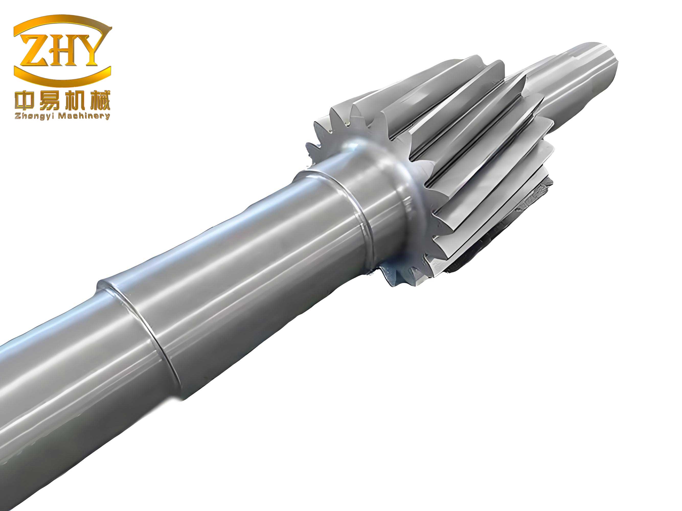
1. Problem Definition and Static Stress Analysis of the Gear Shaft
The subject of this study is a high-speed helical gear shaft that experienced catastrophic fatigue fracture in service. The failure occurred at a specific geometric feature, indicating a probable stress concentration site. The primary objective of the initial analysis phase is to determine the stress distribution under maximum operational loading and identify critical locations.
1.1 Finite Element Model Development and Material Properties
A three-dimensional solid model of the helical gear shaft is developed, incorporating key features such as bearing journals, the helical gear mesh section, keyways, and threaded sections with relief grooves. The model is appropriately simplified by suppressing non-critical details like small fillets and chamfers that do not significantly influence global stress patterns. The material for the gear shaft is a high-strength alloy steel, commonly used for such demanding applications. Its essential mechanical properties are summarized in Table 1.
| Property | Symbol | Value | Unit |
|---|---|---|---|
| Elastic Modulus | E | 208 | GPa |
| Poisson’s Ratio | ν | 0.295 | – |
| Tensile Yield Strength | σ_y | 785 | MPa |
| Ultimate Tensile Strength | σ_u | 980 | MPa |
The static allowable stress, considering a safety factor $n_s = 1.3$, is calculated as:
$$[\sigma] = \frac{\sigma_y}{n_s} = \frac{785}{1.3} \approx 604 \text{ MPa}$$
1.2 Load Application and Boundary Conditions
The gear shaft is analyzed under the most severe in-service loading condition. The loads are applied as follows:
- Torque Input: The torque from the drive motor is applied as a tangential force distribution on the sides of the input keyway.
- Gear Mesh Forces: The reaction from the mating helical gear is applied as a distributed normal force on the gear tooth face, resolved into tangential, radial, and axial components.
- Boundary Conditions: The support locations at the bearing journals are constrained in all translational degrees of freedom to simulate the static support condition.
The resulting static stress field, represented by the von Mises equivalent stress, is computed using the finite element method. The analysis reveals a distinct stress concentration. The maximum equivalent stress, $\sigma_{max} = 431.5 \text{ MPa}$, is localized at the transition region between a shaft shoulder and the adjacent thread relief groove near the input end. Crucially, this location coincides precisely with the site of the actual physical fracture observed on the failed gear shaft. While this peak stress is below the material’s yield strength and the calculated allowable stress of 604 MPa, its localized nature under a cyclic load regime is the initiating factor for fatigue damage. This confirms that the failure mode is high-cycle fatigue, not static overload.
2. Fatigue Life Assessment Methodology
Fatigue failure occurs under cyclic stresses significantly lower than the ultimate tensile strength of the material. The prediction of fatigue life for the gear shaft requires three fundamental inputs: the detailed stress field from the FE model, the cyclic material properties, and an accurate representation of the operational load history.
2.1 Cyclic Material Data and Damage Accumulation
The fatigue resistance of the material is characterized by an S-N curve (Stress vs. Number of cycles to failure). For the alloy steel of the gear shaft, this curve can be estimated using the Seeger method based on the ultimate tensile strength. The linear cumulative damage rule (Palmgren-Miner rule) is employed to assess life under variable amplitude loading. The rule states that failure occurs when the sum of cycle fractions equals 1:
$$D = \sum_{i=1}^{k} \frac{n_i}{N_i} = 1$$
where $D$ is the total damage, $n_i$ is the number of cycles endured at a specific stress level $i$, and $N_i$ is the number of cycles to failure at that same stress level as per the material’s S-N curve.
2.2 Derivation of the Operational Load Spectrum
A critical and complex step is defining the load time-history the gear shaft experiences. For the tilting mechanism, the load is derived from the tilting torque of the vessel, which varies with its angular position and the specific process operation (charging, tapping, slagging, etc.). The torque $M_{tilt}$ at the vessel is transmitted to the high-speed gear shaft torque $T_{shaft}$ through the total gear ratio $p$ and number of motors $n_1$:
$$T_{shaft} = \frac{M_{tilt}}{p \cdot n_1} \cdot \eta$$
where $\eta$ represents the drive efficiency. For analysis purposes, this relationship is simplified to a proportional constant $K$ based on the system’s rated parameters: $T_{shaft} = K \cdot M_{tilt}$.
A full production cycle is analyzed, and the tilting torque is calculated for key operational stages. The most demanding torque values (positive and negative) for dynamic operations like tapping and charging are used, while steady-state stages like blowing use an average value. This leads to a simplified, conservative block load spectrum for one production cycle, as detailed in Table 2.
| Process Stage | Motor Active Time (min) | Shaft Torque, $T_{shaft}$ (Nm) | Cycles at 500 rpm |
|---|---|---|---|
| Tapping / Slagging | 2.40 | +1090.1 | 1200 |
| Return from Tap | 0.25 | -479.3 | 125 |
| Charging | 0.38 | +428.0 | 190 |
| Return from Charge | 0.19 | -339.4 | 95 |
| Positioning | 0.20 | +861.8 | 100 |
| Sampling | 0.60 | -1055.8 | 300 |
| Final Return | 0.30 | +1055.8 | 150 |
This sequence of torque blocks, constituting one load cycle, is repeated for the entire service life of the gear shaft.
3. Fatigue Life Calculation and Results
The fatigue analysis is performed using a dedicated post-processor (FE-SAFE) coupled with the static FEA results. The stress tensor history for every node in the model is scaled according to the load spectrum from Table 2. The von Mises stress with a Goodman mean stress correction is used in conjunction with the material’s S-N curve and the Miner’s rule to compute the fatigue life at every point on the gear shaft.
3.1 Life Distribution and Critical Location
The primary output is a contour plot of the logarithm of fatigue life (log N). The analysis unequivocally identifies the region of minimum fatigue life. The most critical location, predicted to have the shortest life, is exactly the same stress concentration zone identified in the static analysis: the thread relief groove transition near the input end. The predicted minimum life is:
$$N_{min} = 10^{5.377} \approx 238,000 \text{ cycles of the load spectrum}.$$
Given the motor speed of 500 rpm and the total active motor time per production cycle (sum of active times in Table 2 is ~4.32 minutes, equivalent to 2160 motor revolutions or 4.32 min of runtime), we can estimate the total operational time until the predicted initiation of a fatigue crack:
$$\text{Time to Crack Initiation} = \frac{N_{min} \times \text{Cycle Active Time}}{60} = \frac{238,000 \times 4.32}{60} \approx 17,100 \text{ hours}.$$
This calculated life must be considered in the context of the applied simplifications and safety factors, but it provides a quantitative basis for inspection intervals.
3.2 Fatigue Safety Factor Map
An alternative and often more intuitive result is the map of fatigue safety factor (FSF). The FSF is defined at each point as the ratio of the endured stress amplitude (from the S-N curve at the required life) to the actual applied stress amplitude. A value below 1.0 indicates insufficient life. The minimum FSF on the gear shaft is found to be approximately 0.73, located at the same critical groove. This value, being significantly less than 1.0, provides clear and direct evidence of the structural inadequacy of the current design under the given cyclic loading, confirming the root cause of the field failure.
4. Discussion and Pathways for Structural Optimization of Gear Shafts
The synergistic application of static FEA and fatigue analysis has successfully diagnosed the failure mechanism. The fracture of the helical gear shaft was initiated by high-cycle fatigue at a pronounced stress concentrator. The following design optimization strategies for such gear shafts can be derived:
- Geometric Optimization at Stress Raisers: The primary focus must be on redesigning the thread relief groove and shaft shoulder transition. This can involve:
- Increasing the radius of the fillet at the groove root to the maximum permissible value.
- Implementing a full undercut or “run-out” groove designed specifically for fatigue reduction.
- Utilizing a continuous, smooth profile change rather than an abrupt step.
The effect of a larger fillet radius $r$ on the theoretical stress concentration factor $K_t$ for a shoulder can be approximated by empirical formulas, generally showing that $K_t$ decreases as $r$ increases.
- Surface Enhancement Techniques: Since fatigue cracks usually initiate at the surface, improving the surface integrity of the gear shaft at critical locations is highly beneficial.
- Shot Peening: Induces compressive residual surface stresses, effectively increasing the fatigue strength. The improvement can be estimated by adding the compressive stress $\sigma_{res}$ to the mean stress in the Goodman correction.
- Surface Rolling/Nitriding: Similar to peening, these processes create a hard, compressively stressed surface layer.
- Material Upgrade: While the current material is high-strength, switching to a variant with higher fracture toughness or a cleaner microstructure (e.g., vacuum remelted steel) can improve resistance to crack initiation and propagation.
- Load Spectrum Refinement: A more accurate, measured load spectrum, rather than a simplified block program, would allow for a more precise life prediction and potentially reveal opportunities for operational changes to reduce extreme loads.
5. Conclusion
This integrated engineering analysis demonstrates a robust methodology for addressing fatigue failures in critical power transmission components like helical gear shafts. The process begins with a detailed static finite element analysis to locate stress concentrations, which for the studied gear shaft was the thread relief groove. Subsequently, a fatigue life assessment, incorporating a realistic operational load spectrum and material cyclic properties, quantitatively predicted a finite life and a fatigue safety factor below 1.0 at that exact location, validating the field observation. The convergence of the static stress hotspot and the minimum fatigue life location provides irrefutable diagnostic evidence. The findings underscore that for dynamically loaded gear shafts, a design that is safe under static loading can still be vulnerable to fatigue failure. The analysis directly points to geometric optimization of stress-concentrating features as the most effective strategy for enhancing the durability and reliability of such gear shafts, providing a clear technical basis for redesign and preventive maintenance scheduling.