
In the field of high-speed and heavy-duty power transmission, the herringbone gear is widely employed because of its excellent load-carrying capacity, balanced axial thrust, and high transmission stability. The actual operating condition of a herringbone gear, however, differs considerably from the ideal meshing assumption. Installation errors such as shaft misalignment, bearing clearance, and the deformation of the pinion shaft under torque inevitably produce a non-uniform load distribution along the tooth width. In many practical applications, the transmitted load is not constant but follows a spectrum of distinct operating conditions. The combined effect of variable load, installation errors, and shaft deformation is a major challenge in the design and life prediction of high-performance herringbone gear sets. In this article, I present a systematic method for analyzing the fatigue performance of a herringbone gear under variable load and actual working conditions. The method includes a finite element contact analysis model that accounts for installation errors and shaft deformation, calculation of the partial load distribution, determination of the maximum contact stress for each load step, and finally the evaluation of the contact strength safety factor based on the load spectrum and the linear cumulative damage rule.
Gear Geometry and Basic Parameters
The herringbone gear set investigated in the present work is located in the last stage of a main drive chain. The gear pair is composed of a pinion denoted as \(z_3\) and a gear denoted as \(z_4\). Both gears are made of high-strength chromium-nickel alloy steel with an elastic modulus \(E = 210\ \mathrm{GPa}\), Poisson’s ratio \(\mu = 0.28\), and a tensile strength limit of approximately \(1100\ \mathrm{MPa}\). The material has sufficient hardness and wear resistance, and it exhibits good hot and cold workability. The basic design parameters of the \(z_3/z_4\) pair are summarized in Table 1.
| Parameter | Pinion \(z_3\) | Gear \(z_4\) |
|---|---|---|
| Normal module (mm) | 3.8 | 3.8 |
| Number of teeth | 25 | 119 |
| Normal pressure angle (°) | 20 | 20 |
| Helix angle (°) | 25 | 25 |
| Single-side face width (mm) | 48 | 48 |
| Recess width (mm) | 23 | 23 |
| Profile shift coefficient | 0.05 | −0.05 |
| Normal addendum coefficient | 1.2 | 1.2 |
| Normal dedendum coefficient | 0.4 | 0.4 |
The effective transverse pressure angle can be obtained from the normal pressure angle and the helix angle using the following relation:
$$
\tan\alpha_{\mathrm{t}} = \frac{\tan\alpha_{\mathrm{n}}}{\cos\beta}
$$
Substituting \(\alpha_{\mathrm{n}} = 20^\circ\) and \(\beta = 25^\circ\) yields \(\alpha_{\mathrm{t}} \approx 21.88^\circ\). This transverse pressure angle is used in the calculation of the helix slope errors caused by bearing clearances and coaxiality errors.
Because the herringbone gears in this drive train have a thin web structure, they are more sensitive to abrupt changes of mesh stiffness and to load-induced deformation. A sudden change in the mesh stiffness or a severe deformation can excite strong vibration and may eventually lead to tooth failure. To reduce the mesh stiffness variation, to minimize the impact due to base-pitch errors and load-induced deformation, and to avoid edge contact and stress concentration, both profile modification and longitudinal crowning modification are applied. Table 2 lists the modification details for \(z_3\) and \(z_4\).
| Gear | Modification type | Amount (μm) |
|---|---|---|
| \(z_3\) left/right hand | Profile modification | 22 |
| \(z_3\) left/right hand | Maximum helix crowning modification | 27 |
| \(z_4\) left/right hand | Profile modification | 19 |
| \(z_4\) left/right hand | Maximum helix crowning modification | 27 |
Finite Element Contact Analysis Model
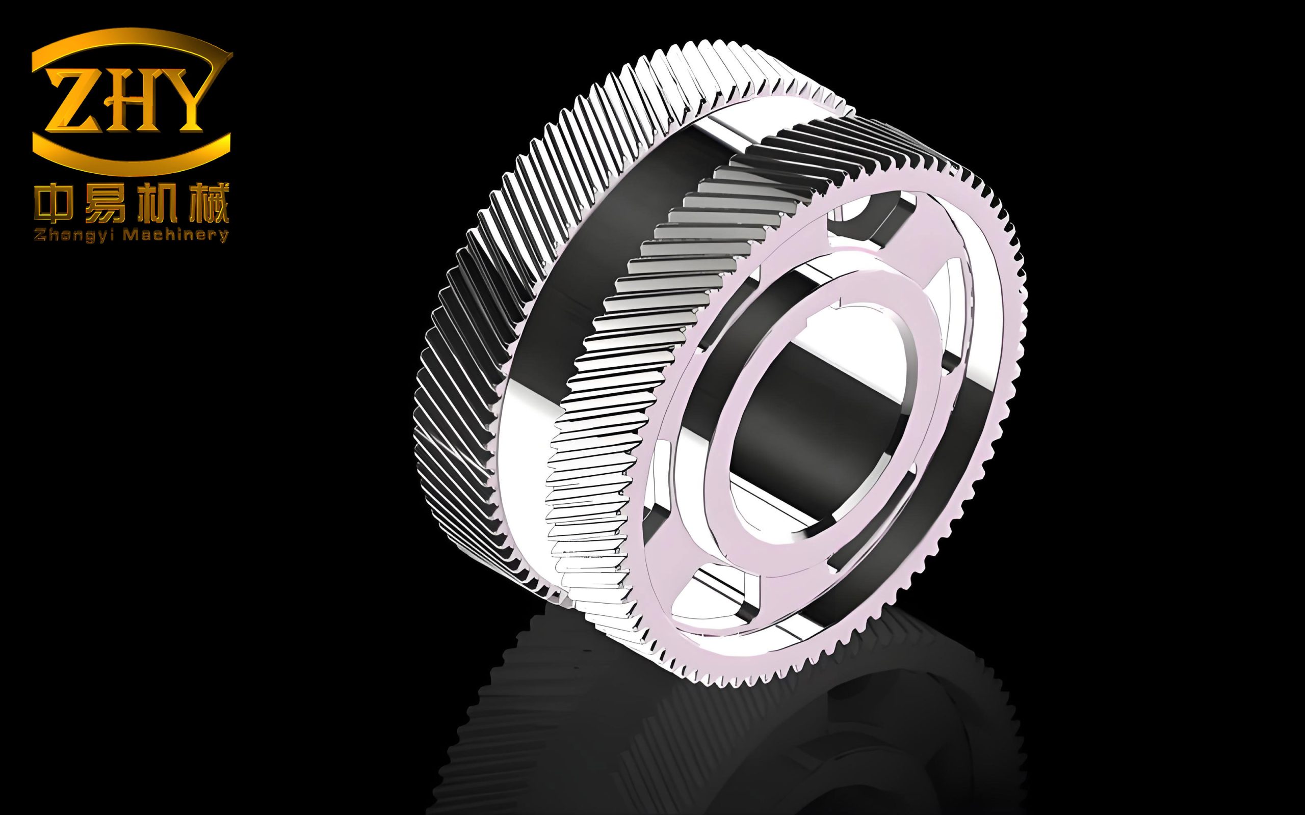
Accurate three-dimensional geometry of the modified herringbone gear is the most important prerequisite for a reliable contact analysis. I generated the modified tooth surface by solving the rack cutter equation and using the envelope principle. The tooth root transition curve was included in the derivation. Then, according to the grinding principle for modified gears, the mathematical model of the modified tooth flank was obtained. By programming in MATLAB and using the secondary development of CATIA through Visual Basic, the modified tooth surface was automatically generated. After circular array and blank cutting, the complete three-dimensional herringbone gear model with compound modification was created. A typical herringbone gear manufactured with a modified tooth flank is illustrated below.
The mesh quality and density greatly influence the accuracy of the finite element contact analysis. A too fine mesh requires excessive computational resources, while a too coarse mesh cannot capture the actual contact stress. Because the herringbone gear has a total contact ratio greater than three, two to three complete meshing cycles should be covered in the simulation. In order to reduce the calculation cost while retaining sufficient accuracy, I adopted a nine-tooth sector model for each gear. The element type is the eight-node linear brick element C3D8R. The final mesh models of \(z_3\) and \(z_4\) are shown in the following sections of this analysis; the mesh at the tooth root and the contact area is locally refined to improve the accuracy of the contact stress computation.
Modeling of Installation Errors and Shaft Deformation
In actual operation, the bearing clearances and the coaxiality errors of the bearing bores and gear shafts produce an angular misalignment between the two gear axes. In addition, the pinion shaft is subjected to bending and torsional moments caused by the helical gear forces. Under heavy load, the shaft deformation can change the relative position of the gears and therefore aggravate the non-uniform load distribution. To obtain a realistic contact stress distribution, I included both installation errors and shaft deformation in the finite element model.
The bearing arrangement of the \(z_3/z_4\) gears is characterized by the bearing center distances \(L_1 = 200.3\ \mathrm{mm}\) and \(L_2 = 374.3\ \mathrm{mm}\). The total face width of the herringbone gear is \(b_m = 119\ \mathrm{mm}\). The equivalent cumulative clearances at the four bearing positions are denoted by \(\delta_1\), \(\delta_2\), \(\delta_3\), and \(\delta_4\). These values include the bearing bore coaxiality error and the gear shaft coaxiality error, as summarized in Table 3.
| Bearing | Bearing bore coaxiality error ε (μm) | Gear shaft coaxiality error φ (μm) | Cumulative clearance (ε+φ)/2 (μm) |
|---|---|---|---|
| \(\delta_1\) | 15 | 6 | 10.5 |
| \(\delta_2\) | 15 | 6 | 10.5 |
| \(\delta_3\) | 0 | 0 | 0 |
| \(\delta_4\) | 15 | 0 | 7.5 |
Using the method reported in the literature, the maximum helix slope errors caused by the spatial geometric factors can be calculated. In the vertical plane, the error of the pinion shaft is:
$$
f_{p\mathrm{I}1} = b_m \frac{\delta_1 + \delta_2}{L_1} \cos\alpha_{\mathrm{t}} = 11.5775\ \mu\mathrm{m}
$$
In the vertical plane, the error of the gear shaft is:
$$
f_{p\mathrm{I}2} = b_m \frac{\delta_3 + \delta_4}{L_2} \cos\alpha_{\mathrm{t}} = 2.2127\ \mu\mathrm{m}
$$
In the axial plane, the error of the pinion shaft is:
$$
f_{p\parallel 1} = b_m \frac{\delta_1 + \delta_2}{L_1} \sin\alpha_{\mathrm{t}} = 4.6497\ \mu\mathrm{m}
$$
In the axial plane, the error of the gear shaft is:
$$
f_{p\parallel 2} = b_m \frac{\delta_3 + \delta_4}{L_2} \sin\alpha_{\mathrm{t}} = 0.8886\ \mu\mathrm{m}
$$
The total helix slope errors in the two directions are therefore:
$$
f_{p\mathrm{I}} = f_{p\mathrm{I}1} + f_{p\mathrm{I}2} = 13.7902\ \mu\mathrm{m}
$$
$$
f_{p\parallel} = f_{p\parallel 1} + f_{p\parallel 2} = 5.5383\ \mu\mathrm{m}
$$
The maximum angular misalignments corresponding to these two errors are:
$$
\theta_x = \arctan\left( \frac{f_{p\mathrm{I}}}{\cos\alpha_{\mathrm{t}} \times 1000 \times b_m} \right) \times \frac{180}{\pi} = 0.0072^\circ
$$
$$
\theta_y = \arctan\left( \frac{f_{p\parallel}}{\sin\alpha_{\mathrm{t}} \times 1000 \times b_m} \right) \times \frac{180}{\pi} = 0.0072^\circ
$$
Thus, the pinion axis is rotated by \(0.0072^\circ\) about the \(x\)-axis, which represents the installation error in the plane of the two gear axes, and by \(0.0072^\circ\) about the \(y\)-axis, which represents the installation error perpendicular to that plane. The standard assembly relationship is then modified according to these rotations. The coordinates of the reference points on the pinion center line are transformed using the rotation matrix. The final reference point coordinates after introducing the installation errors are denoted by \(R_{p2}’\) and \(R_{p3}’\).
The torsional deformation of the pinion shaft is introduced in the boundary conditions. The finite element simulation is divided into four implicit static analysis steps:
Step 1: The reference point \(R_{p1}\) for the gear and the two reference points \(R_{p2}’\), \(R_{p3}’\) for the pinion are constrained in all degrees of freedom. A small rotation is applied to the pinion reference point \(R_{p2}’\) to remove clearances caused by mesh generation and modeling errors, while the rotation of \(R_{p3}’\) about the axis is released.
Step 2: The rotational degree of freedom of \(R_{p2}’\) is released, and a small torque is applied to \(R_{p2}’\) to establish stable contact and to ensure convergence of the analysis.
Step 3: The reference point \(R_{p2}’\) is coupled with the end surface of the pinion shaft, and the rated torque is applied. In this way, the torsional deformation of the pinion shaft is naturally included in the contact simulation.
Step 4: The gear reference point \(R_{p1}\) is rotated by the angle corresponding to nine tooth pitches, which gives a complete meshing cycle for the nine-tooth sector model.
Load Spectrum and Contact Stress Results
The actual service load of the \(z_3/z_4\) herringbone gear pair is not constant. Table 4 presents the measured load spectrum, which consists of six typical operating conditions. Conditions 1 to 4 occupy 73.3% of the total operating time and have relatively high input power levels around 3000 kW. The maximum input power is 3781 kW in the first condition.
| Condition | Input power (kW) | Torque of \(z_3/z_4\) (N·m) | Output speed (r/min) | Time proportion (%) |
|---|---|---|---|---|
| 1 | 3781 | 4050.062 | 1020 | 3.42 |
| 2 | 2943 | 3782.914 | 850 | 1.32 |
| 3 | 3026 | 3673.513 | 900 | 51.23 |
| 4 | 3403 | 3645.163 | 1020 | 17.33 |
| 5 | 883 | 1135.003 | 850 | 12.62 |
| 6 | 69 | 376.941 | 7200 | 14.00 |
For each operating condition, I applied the corresponding torque to the finite element model and performed a quasi-static contact analysis. The maximum contact stress on the left-hand and right-hand tooth flanks of both gears was extracted over one complete meshing cycle. Table 5 lists the results when installation errors and shaft deformation are included. Table 6 lists the corresponding results for the ideal case without installation errors and shaft deformation.
| Condition | \(z_3\) left flank | \(z_3\) right flank | \(z_4\) left flank | \(z_4\) right flank |
|---|---|---|---|---|
| 1 | 1255 | 1188 | 1153 | 1277 |
| 2 | 1221 | 1161 | 1122 | 1193 |
| 3 | 1208 | 1149 | 1107 | 1174 |
| 4 | 1203 | 1146 | 1106 | 1170 |
| 5 | 794 | 763 | 698 | 736 |
| 6 | 525 | 495 | 418 | 448 |
| Condition | \(z_3\) left flank | \(z_3\) right flank | \(z_4\) left flank | \(z_4\) right flank |
|---|---|---|---|---|
| 1 | 1239 | 1239 | 1200 | 1200 |
| 2 | 1206 | 1206 | 1164 | 1164 |
| 3 | 1192 | 1192 | 1148 | 1148 |
| 4 | 1188 | 1188 | 1144 | 1144 |
| 5 | 783 | 783 | 717 | 717 |
| 6 | 516 | 516 | 432 | 432 |
By comparing the two tables, I found that the load sharing between the left-hand and right-hand flanks of the herringbone gear is significantly affected by installation errors and shaft deformation. In the most severe condition, the difference between the left and right flank maximum contact stresses reaches 124 MPa. In relative terms, the maximum deviation of the load sharing is 10.75%. This partial load would reduce the fatigue life of the more heavily loaded flank and must be considered in the fatigue design of the herringbone gear.
Contact Strength Safety Factor under Variable Load
To quantify the fatigue performance of the herringbone gear, I calculated the contact strength safety factor according to the variable-load design method in the gear transmission design handbook. The calculation is based on the linear cumulative damage theory. For a given stress level \(\sigma_i\), the fatigue damage is defined as the ratio of the number of actual stress cycles \(N_{Li}\) to the number of cycles to failure \(N_i\) read from the S–N curve. The total fatigue damage \(U\) is the sum of the individual damage fractions:
$$
U = \sum U_i = \sum \frac{N_{Li}}{N_i}
$$
For contact strength, the S–N curve can be expressed in the form:
$$
\sigma_1 = \sigma_2 \left( \frac{N_2}{N_1} \right)^{1/(2p)}
$$
where \(p\) is the material fatigue curve exponent, which depends on the material, heat treatment, and the working cycle range. The values used in the present analysis are listed in Table 7.
| Allowable pitting | Cycle range \(N_L\) | \(p\) |
|---|---|---|
| Pitting allowed | \(6 \times 10^5 < N_L \le 10^7\) | 6.77 |
| \(10^7 < N_L \le 10^9\) | 8.78 | |
| \(10^9 < N_L \le 10^{10}\) | 7.08 | |
| Pitting not allowed | \(10^5 < N_L \le 5 \times 10^7\) | 6.61 |
| \(5 \times 10^7 < N_L \le 10^{10}\) | 16.30 |
For the gear material under investigation, the contact fatigue strength at \(10^7\) cycles is 1600 MPa. The total fatigue damage can then be written in terms of the applied stress \(\sigma_i\) and the corresponding exponent \(p_i\):
$$
U = \sum U_i = \sum \frac{N_{Li}}{10^7} \left( \frac{\sigma_i}{1600} \right)^{2p_i}
$$
After obtaining the total fatigue damage \(U\), the contact strength safety factor \(S_H\) is calculated as:
$$
S_H = \frac{1}{U^{\,1/(2p_i)}}
$$
In the above expression, the exponent \(p_i\) is selected according to the cycle range of the corresponding load condition. The number of stress cycles \(N_{Li}\) for each condition is determined from the output speed and the time proportion within the expected service life of 1000 h. I computed the cycle counts for each load step and then substituted the maximum contact stress from either Table 5 or Table 6 into the damage equation. The resulting safety factors are summarized in Table 8.
| Herringbone gear | \(S_H\) without errors and deformation | \(S_H\) with errors and deformation |
|---|---|---|
| Pitting allowed | ||
| \(z_3\) | 1.124 | 1.110 |
| \(z_4\) | 1.264 | 1.226 |
| Pitting not allowed | ||
| \(z_3\) | 1.065 | 1.059 |
| \(z_4\) | 1.249 | 1.216 |
When installation errors and shaft deformation are taken into account, the safety factor of the \(z_3\) tooth flank decreases by 1.25% if a limited amount of pitting is allowed, and by 0.56% if pitting is not allowed. For the \(z_4\) gear, the corresponding reductions are 3.01% and 2.64%. The larger decrease in the safety factor of \(z_4\) indicates that the right flank of \(z_4\) is more severely affected by the partial load. This observation suggests that the current modification design of the herringbone gear still has room for optimization.
Discussion
The numerical results confirm that the fatigue performance of a herringbone gear cannot be accurately evaluated by an ideal no-error model. The installation error of \(0.0072^\circ\) in each direction appears to be very small, but its effect on the contact stress distribution is noticeable. Since the herringbone gear has a large face width, even a small angular misalignment causes a significant helix slope mismatch between the left-hand and right-hand tooth flanks. Consequently, one flank carries a higher portion of the load, leading to a higher local contact stress and a lower safety factor.
Shaft deformation is another important factor. The torque applied to the pinion shaft causes a torsional twist along the shaft. Because the finite element model couples the reference point to the shaft end, the twist is transmitted to the gear body and changes the actual meshing position along the face width. In a multi-stage transmission, the shaft is usually supported by multiple bearings, and the deformation is not uniform. The method presented here can quantitatively capture this effect and provides a useful reference for the design and analysis of high-performance herringbone gear sets.
The variable load spectrum is essential for a realistic fatigue life estimation. A single constant load analysis would overestimate or underestimate the damage depending on the chosen load level. The linear cumulative damage rule combined with the actual load spectrum gives a straightforward safety factor that can be used in engineering design. The safety factor values in Table 8 are close to unity, indicating that the gear pair is designed near its fatigue limit. Therefore, the modification parameters should be optimized to reduce the partial load and to improve the fatigue life of the herringbone gear.
Conclusion
In this article, I have developed a complete finite-element-based method for analyzing the fatigue performance of a herringbone gear under variable load and actual working conditions. The method can be summarized in the following steps. First, a precise three-dimensional model of the modified herringbone gear is generated from the rack cutter envelope and the grinding modification principle. Second, installation errors and shaft deformation are introduced into the boundary conditions of the finite element model. Third, quasi-static contact analyses are performed for each load step of the measured load spectrum. Finally, the contact strength safety factor is calculated using the linear cumulative damage theory. The practical application of the proposed method to a \(z_3/z_4\) herringbone gear pair shows that the maximum load sharing difference between the left-hand and right-hand flanks is 124 MPa, which corresponds to a relative deviation of 10.75%. When installation errors and shaft deformation are considered, the contact strength safety factor of the \(z_4\) gear decreases by 3.01% in the pitting-allowed case. This indicates that the current modification design of the herringbone gear can be further improved to reduce the sensitivity of the gear pair to installation errors and shaft deformation. The proposed approach provides a useful engineering tool for the fatigue design and modification optimization of high-performance herringbone gears.