
In modern mechanical engineering, the design of critical components like gear shafts must account for the inherent uncertainties in loads, material properties, and manufacturing processes. Traditional design methods often rely on deterministic safety factors, which may not adequately capture the probabilistic nature of fatigue failure. As an engineer focused on reliability, I aim to explore the fatigue reliability design methodology for gear shafts, which are subjected to combined bending and torsional stresses in applications such as reducers. This approach treats fatigue failure as a random event, incorporating the dispersions in stress, strength, and influencing factors through probabilistic models. By leveraging stress-strength interference theory and considering variables like stress concentration, size effects, and surface conditions as probability distributions, we can achieve a more robust and safer design for gear shafts. This article will delve into the theoretical foundations, computational steps, and a practical example, emphasizing the use of formulas and tables to summarize key concepts. Throughout, the term ‘gear shaft’ will be highlighted to underscore its central role in power transmission systems.
The transition from conventional fatigue design to reliability-based design marks a significant paradigm shift. In traditional methods, the S-N curve represents a 50% reliability level, ignoring the variability in both applied stresses and material strength. For a gear shaft operating under cyclic loads, this oversight can lead to unexpected failures, especially in high-performance systems like automotive reducers. Reliability design, however, models loads, material strengths, and geometric dimensions as statistical quantities with specific probability distributions. This allows us to establish relationships between stress, strength, and reliability using probability and statistical theory. Consequently, we can perform cross-sectional design, compute reliability indices, or select appropriate materials with a quantifiable confidence level. The gear shaft, as a rotating shaft enduring both bending moments and torques, is a prime candidate for this methodology, as its failure mode—fatigue fracture—is highly sensitive to stochastic variations.
Fatigue strength in reliability design is characterized by probabilistic distributions rather than single values. The P-S-N curve, which plots stress against cycles for different reliability levels, illustrates this concept. For instance, the curve for R=50% corresponds to the conventional S-N curve, while those for R=90% or R=99% represent higher survival probabilities. At a given stress ratio r, the fatigue limit at a specified life (e.g., N > 10^7 cycles) is not a fixed value but follows a distribution, forming a three-dimensional surface when combined with various r values. This complexity arises because both the fatigue strength of the material and the working stresses on the gear shaft exhibit dispersions. To visualize this, consider the fatigue strength probability distribution diagram, where for each r, the fatigue limit is represented as a distribution band. This probabilistic framework is crucial for accurately assessing the reliability of a gear shaft under real-world loading conditions.
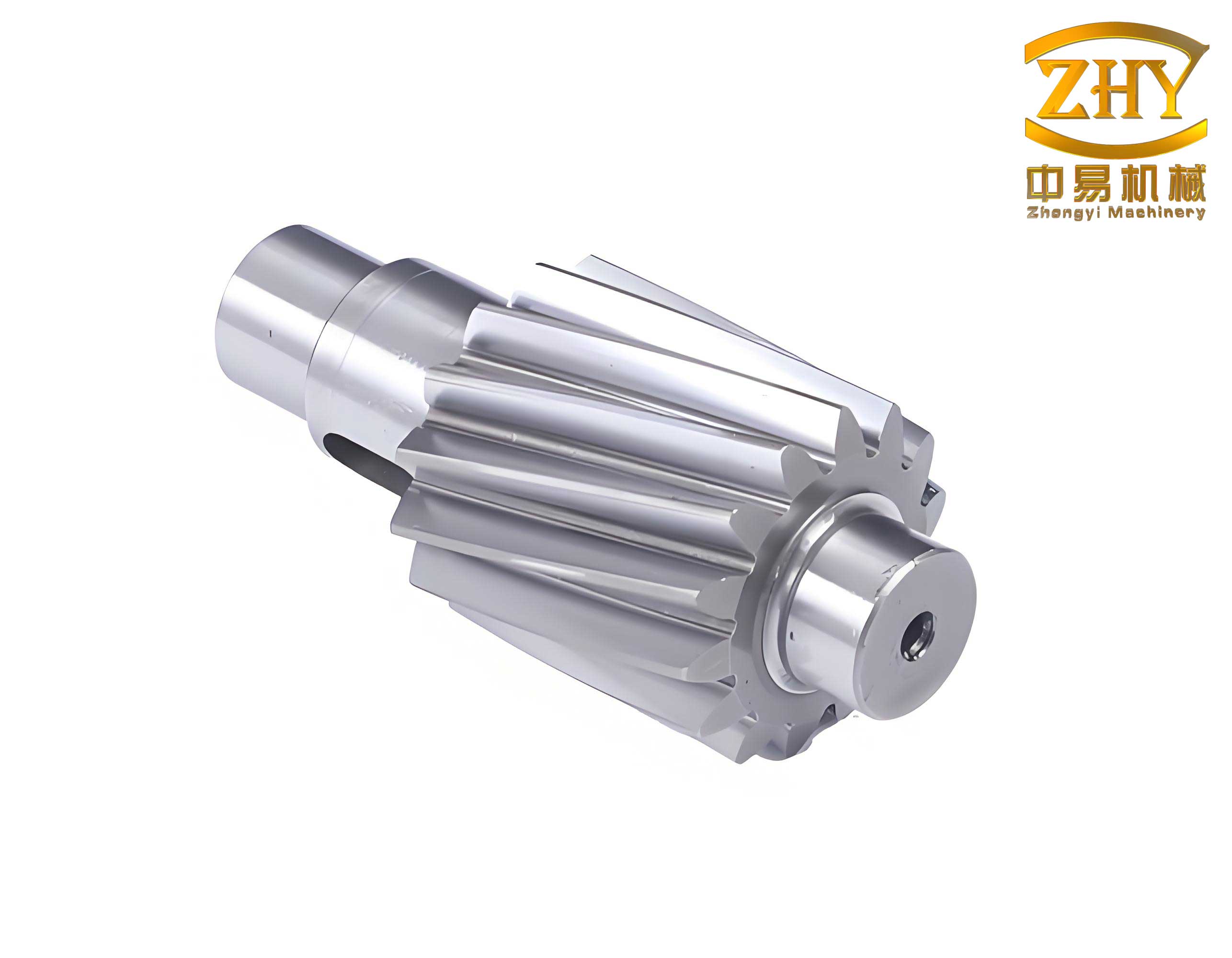
In reliability design, several influence factors must be treated probabilistically, as their variations significantly impact the fatigue performance of a gear shaft. These include the effective stress concentration coefficient, size coefficient, and surface finish coefficient. Unlike conventional design, where these are often taken as deterministic values, we assign them means and standard deviations to reflect their randomness. For example, the effective stress concentration coefficient Kσ accounts for geometric discontinuities like fillets in a gear shaft. Its mean is given by Kσ = 1 + q(Kt – 1), where q is the notch sensitivity mean and Kt is the theoretical stress concentration factor. The standard deviation sK is computed as sK = (Kt – 1)sq, with sq being the standard deviation of q. Similarly, the size coefficient ε, which reduces fatigue strength for larger diameters, and the surface finish coefficient β, which accounts for manufacturing effects, are characterized by their distributions. Tables summarizing typical values for common materials can aid in design. For instance, the table below provides hypothetical data for steel gear shafts:
| Factor | Mean | Standard Deviation | Remarks |
|---|---|---|---|
| Effective Stress Concentration Coefficient (Kσ) | 1.8 | 0.05 | Depends on geometry (e.g., fillet radius) |
| Size Coefficient (ε) | 0.9 | 0.03 | For diameter d > 10 mm |
| Surface Finish Coefficient (β) | 1.1 | 0.02 | For ground gear shafts |
These coefficients are pivotal in transforming the material fatigue limit into the component fatigue limit for a gear shaft. Their probabilistic treatment ensures that the design accounts for real-world variabilities, such as manufacturing tolerances or material batch differences, which are often overlooked in traditional approaches.
To determine the fatigue limit of a gear shaft under different stress ratios r, we need to compute the mean and standard deviation of the stress amplitude and mean stress. For a given r, which is the ratio of minimum to maximum stress (r = σ_min / σ_max), the stress amplitude σ_a and mean stress σ_m are derived from the maximum and minimum stresses. Their means are calculated as:
$$ \bar{\sigma}_a = \frac{\bar{\sigma}_{\text{max}} – \bar{\sigma}_{\text{min}}}{2} $$
$$ \bar{\sigma}_m = \frac{\bar{\sigma}_{\text{max}} + \bar{\sigma}_{\text{min}}}{2} $$
Assuming r is constant, the standard deviations are:
$$ s_a = \frac{1 – r}{2} s_\sigma $$
$$ s_m = \frac{1 + r}{2} s_\sigma $$
where s_σ is the standard deviation of the stress distribution. The fatigue limit mean σ_r and its standard deviation s_r for a specific r are then:
$$ \sigma_r = \sqrt{\bar{\sigma}_a^2 + \bar{\sigma}_m^2} $$
$$ s_r = \sqrt{\frac{\bar{\sigma}_a^2 s_a^2 + \bar{\sigma}_m^2 s_m^2}{\bar{\sigma}_a^2 + \bar{\sigma}_m^2}} $$
These formulas allow us to construct the fatigue limit line diagram for the material, which appears as a distribution band rather than a single curve. For a gear shaft, this diagram is essential for comparing with working stresses in reliability assessments. By plotting these distributions for various r, we can visualize the probabilistic fatigue strength envelope, aiding in the design of a robust gear shaft.
The fatigue limit of the actual gear shaft component is derived from the material fatigue limit by incorporating the influence coefficients. If the material fatigue limit distribution is (σ’_r, s’_σ), then the component fatigue limit (σ_r, s_σ) is given by:
$$ (\sigma_r, s_\sigma) = \frac{(\bar{\epsilon}, s_\epsilon)(\bar{\beta}, s_\beta)}{(\bar{K}_\sigma, s_K)} (\sigma’_r, s’_\sigma) $$
Here, (ε̄, s_ε) is the size coefficient distribution, (β̄, s_β) is the surface finish coefficient distribution, and (K̄_σ, s_K) is the effective stress concentration coefficient distribution. This equation represents a probabilistic scaling of the material properties to account for the gear shaft’s specific geometry and manufacturing. For instance, a gear shaft with a large diameter or a rough surface will have a reduced fatigue limit, and this reduction is modeled with its variability. By computing these distributions, we obtain the fatigue strength distribution of the gear shaft, which is crucial for subsequent reliability calculations.
Reliability computation hinges on the stress-strength interference model, where failure occurs if the stress exceeds the strength. For a gear shaft, we define the stress distribution (x̄_σ, s_σ) from the applied loads and the strength distribution (x̄_s, s_s) from the component fatigue limit. The reliability index z, also known as the coupling coefficient, is calculated as:
$$ z = \frac{\bar{x}_s – \bar{x}_\sigma}{\sqrt{s_s^2 + s_\sigma^2}} $$
This z-value corresponds to the probability of survival (reliability R) under the assumption that both stress and strength follow normal distributions. Using standard normal distribution tables, we can find R for a given z. For example, z = 3.719 corresponds to R ≈ 0.9999. In design, we iteratively adjust the gear shaft dimensions until the computed R meets or exceeds the target reliability, ensuring that the gear shaft can withstand operational uncertainties with high confidence.
To illustrate the application of fatigue reliability design for gear shafts, consider a case study involving a reducer gear shaft similar to the one described earlier. The gear shaft transmits torque and bears bending forces, with potential variations in loads and dimensions. We will walk through the key steps, emphasizing probabilistic calculations. Assume the gear shaft is made of 40CrNiMoA steel, with a required reliability R = 0.9999 for a life N > 10^7 cycles. The shaft is ground, and its preliminary dimensions are based on conventional design. We will focus on a critical cross-section, such as a fillet region, where stress concentration is high.
First, identify the critical point on the gear shaft. Through stress analysis, a fillet with radius R8 might be the most vulnerable due to combined bending and torsion. Next, compute the bending moments from horizontal and vertical forces. Suppose the horizontal force is (30000 ± 1500) N, leading to a bending moment M_h with mean and standard deviation derived from force and distance distributions. For instance, if the distance from bearing to critical section is (495, 1.67) mm, then:
$$ \bar{M}_h = 7425000 \, \text{N·mm}, \quad s_{M_h} = 126000 \, \text{N·mm} $$
Similarly, the vertical moment M_v from forces (15000 ± 750) N might yield:
$$ \bar{M}_v = 3750000 \, \text{N·mm}, \quad s_{M_v} = 63700 \, \text{N·mm} $$
The resultant bending moment M is then:
$$ \bar{M} = \sqrt{\bar{M}_h^2 + \bar{M}_v^2} = 8318000 \, \text{N·mm} $$
$$ s_M = \sqrt{\frac{\bar{M}_h^2 s_{M_h}^2 + \bar{M}_v^2 s_{M_v}^2}{\bar{M}_h^2 + \bar{M}_v^2}} = 116000 \, \text{N·mm} $$
The torque T on the gear shaft is assumed as (4430000, 73833) N·mm. With the shaft diameter d = (105, 0.525) mm, the bending stress σ and torsional stress τ are computed using section modulus formulas. For a circular gear shaft cross-section:
$$ \bar{\sigma} = \frac{\bar{M}}{(\pi/32) \bar{d}^3}, \quad s_\sigma \approx \sqrt{\left(\frac{\partial \sigma}{\partial M}\right)^2 s_M^2 + \left(\frac{\partial \sigma}{\partial d}\right)^2 s_d^2} $$
Using probabilistic algebra, we might get σ̄ = 73.19 MPa and s_σ = 1.499 MPa. Similarly, for torsion:
$$ \bar{\tau} = \frac{\bar{T}}{(\pi/16) \bar{d}^3}, \quad s_\tau = 0.437 \, \text{MPa} $$
The combined stress σ_f using von Mises criterion is:
$$ \bar{\sigma}_f = \sqrt{\bar{\sigma}^2 + 3\bar{\tau}^2} = 80.6 \, \text{MPa} $$
$$ s_{\sigma_f} = \sqrt{\frac{\bar{\sigma}^2 s_\sigma^2 + 9\bar{\tau}^2 s_\tau^2}{\bar{\sigma}^2 + 3\bar{\tau}^2}} = 1.4 \, \text{MPa} $$
This represents the working stress distribution on the gear shaft for a specific stress ratio r, which in this case is around -0.369 (indicating alternating stresses).
Next, determine the material fatigue limit distribution from test data. For 40CrNiMoA steel at N = 10^7 cycles, we might have:
- At r = -1: σ̄’_r = 534 MPa, s’_r = 20.0 MPa
- At r = 0.1: σ̄’_r = 1050 MPa, s’_r = 33.3 MPa
Using interpolation for r = -0.369, we compute the stress amplitude and mean stress distributions, then apply the influence coefficients. For the gear shaft, with K̄_σ = 1.82, s_K = 0.0384 (based on q and K_t), ε̄ = 0.494, s_ε = 0.0447, and β̄ = 1.0 (since ground), the component fatigue limit is scaled as per earlier equation. Assuming calculations yield:
$$ \bar{x}_s = 272.9 \, \text{MPa}, \quad s_s = 21.5 \, \text{MPa} $$
This is the strength distribution of the gear shaft at the critical point. Now, compute the reliability index z:
$$ z = \frac{272.9 – 80.6}{\sqrt{21.5^2 + 1.4^2}} = 8.925 $$
This z-value corresponds to an extremely high reliability R > 0.99999999, indicating that the preliminary gear shaft design is overly conservative. We can iteratively reduce dimensions to achieve a target R ≈ 0.9999, optimizing the gear shaft for weight and cost while maintaining safety.
The table below summarizes key probabilistic parameters for this gear shaft example:
| Parameter | Mean | Standard Deviation | Units |
|---|---|---|---|
| Bending Moment M | 8.318e6 | 1.16e5 | N·mm |
| Shaft Diameter d | 105 | 0.525 | mm |
| Bending Stress σ | 73.19 | 1.499 | MPa |
| Torsional Stress τ | 19.49 | 0.437 | MPa |
| Combined Stress σ_f | 80.6 | 1.4 | MPa |
| Material Fatigue Limit (r=-1) | 534 | 20.0 | MPa |
| Component Fatigue Limit | 272.9 | 21.5 | MPa |
| Reliability Index z | 8.925 | — | — |
This iterative process underscores the power of reliability design for gear shafts. By explicitly modeling uncertainties, we can tailor dimensions to meet specific reliability targets, avoiding both over-design and under-design. The gear shaft, as a load-bearing element in reducers, benefits greatly from this approach, as fatigue failures often stem from unaccounted variabilities in manufacturing or operation.
In conclusion, fatigue reliability design for gear shafts offers a superior framework compared to traditional methods by incorporating the probabilistic nature of stresses, strengths, and influence factors. Through the stress-strength interference model, we can compute reliability indices and optimize gear shaft dimensions for desired safety levels. The use of P-S-N curves with distribution bands, probabilistic influence coefficients, and rigorous calculations ensures that designs are both economical and robust. This methodology is not limited to gear shafts in reducers but can be extended to other rotating machinery components, providing a blueprint for reliable engineering in the face of uncertainty. As industries demand higher performance and longer lifetimes, embracing such probabilistic approaches for gear shafts will become increasingly essential.
To further elaborate, consider the mathematical foundations. The probability density functions for stress and strength are often assumed normal for simplicity, but other distributions like log-normal or Weibull can be used for greater accuracy. For a gear shaft under complex loading, Monte Carlo simulations might supplement analytical methods, allowing for the assessment of rare events. Additionally, modern tools like finite element analysis can feed stress distributions into reliability models, enhancing precision. The key is to maintain a holistic view where every variable—from load fluctuations to surface roughness on the gear shaft—is treated as a random quantity. This mindset shift from deterministic to probabilistic design is what ultimately safeguards critical components like gear shafts against unforeseen failures.
In practice, implementing fatigue reliability design for gear shafts requires collaboration across disciplines: materials science for fatigue data, manufacturing for tolerance distributions, and field engineering for load spectra. By integrating these inputs, we can build comprehensive models that predict reliability over the gear shaft’s lifecycle. For instance, in automotive applications, where gear shafts in reducers face varying loads, a reliability-based approach can inform maintenance schedules and design improvements. Ultimately, this leads to safer, more durable products, reinforcing the importance of probabilistic thinking in mechanical design. As we advance, continued research into material behaviors and statistical methods will further refine our ability to design reliable gear shafts for ever-more demanding environments.