
In my extensive experience with heavy machinery manufacturing, the machining of large straight bevel gears presents unique challenges due to their size and low-speed applications. These straight bevel gears are often integral to massive equipment such as mining crushers, wind turbine yaw drives, and marine propulsion systems, where high torque transmission is critical. The traditional method of form milling has remained prevalent for these特大规格 straight bevel gears, primarily because it offers higher production efficiency and lower cost compared to generating methods like gear planing. Moreover, the scarcity of large-scale gear planing machines capable of handling such dimensions makes form milling a practical necessity. This article delves into the fundamental principles, design methodologies, and error compensation techniques I have employed in form milling large straight bevel gears, with a focus on ensuring functional meshing despite the inherent approximations of the process.
The core principle of form milling for straight bevel gears involves using a finger-type milling cutter whose axis intersects the workpiece axis within a common plane. A typical setup, as utilized in machines like the OKU50铣齿机, positions the cutter and gear blank such that the cutter rotates while feeding along a predetermined path relative to the gear. After milling one tooth space, the workpiece is indexed automatically to machine the next, and this cycle repeats for all teeth. A critical adjustable parameter is the angle between the workpiece axis and the feed direction of the cutter, denoted as S. This angle adjustment, often referred to as the setting angle, allows for modification of the cutting depth across the face width of the gear tooth. However, this is where the fundamental limitation arises: a single finger cutter has a fixed profile, meaning it mills identical tooth profiles at both the toe (small end) and heel (large end) of the straight bevel gear. In reality, due to the conical geometry, a straight bevel gear requires progressively larger module (or diametral pitch) from toe to heel. The tooth profile should ideally be an involute that varies along the face width. Therefore, form milling can only produce an approximation of the true conjugate tooth form, leading to what we term as approximate machining. The goal of process design is to minimize the resulting meshing errors to acceptable levels through careful cutter profile design and machining parameter adjustment.
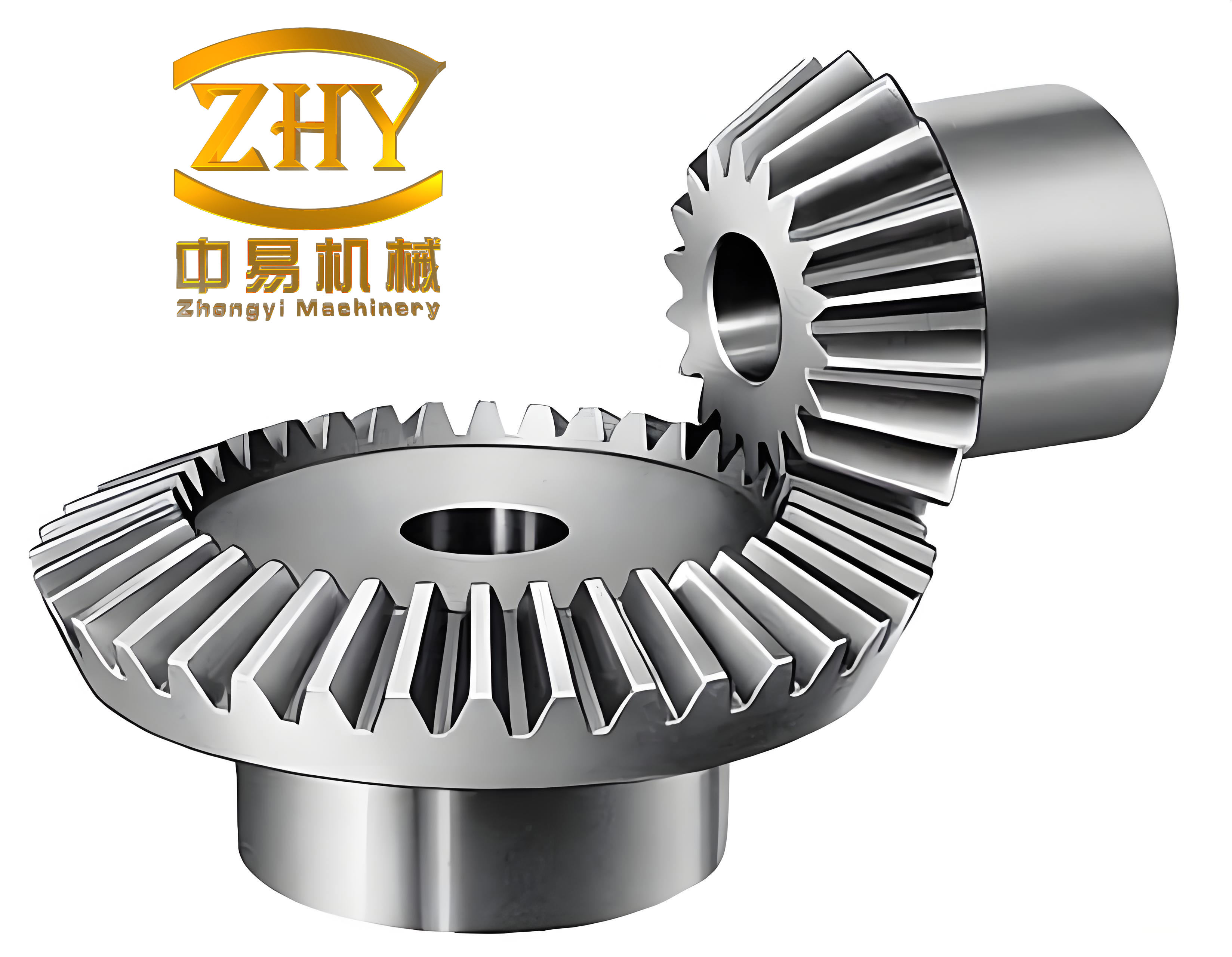
The geometry of a straight bevel gear is defined by several key parameters. Let the mean module at the pitch cone midpoint be \(m\), the number of teeth be \(z\), the pitch cone distance (outer) be \(R\), the face width be \(b\), the addendum coefficient be \(h_a^*\), and the profile shift coefficient be \(x\). The pitch cone angle for the gear in a pair is \(\delta\). For a gear pair, we have the pinion (gear 1) and the wheel (gear 2). The module at any point along the face width is proportional to its distance from the apex. Thus, the module at the small end (toe), \(m_i\), and at the large end (heel), \(m_h\), can be calculated as:
$$ m_i = m \left( \frac{R – b}{R} \right) $$
$$ m_h = m \left( \frac{R + b}{R} \right) $$
In practice, for large straight bevel gears, the variation is significant. To design the cutter profile, we often work with the concept of equivalent spur gear teeth. The equivalent or virtual number of teeth \(z_v\) for a straight bevel gear is given by:
$$ z_v = \frac{z}{\cos \delta} $$
This transformation allows us to use standard spur gear tooth profile calculations as a basis for designing the cutter profile for the straight bevel gear. The primary challenge is selecting a reference module \(m_0\) for which the cutter profile will be generated. Two main design philosophies have been developed: the Mid-Face Module Method and the Paired Design Method. Each has its merits and trade-offs in machining large straight bevel gears.
Mid-Face Module Method: Design and Error Analysis
The Mid-Face Module Method, as the name implies, uses the module at the midpoint of the face width as the reference module \(m_0\) for cutter design. Consequently, the milled tooth profile will be theoretically correct only at this central section of the straight bevel gear. The tooth profiles at the toe and heel will deviate from the ideal, leading to meshing errors. Let me illustrate this with a detailed example using a specific gear pair parameters, which I have encountered frequently in production.
Consider a pair of large straight bevel gears with the following specifications:
- Mean module at pitch cone, \(m = 45 \, \text{mm}\)
- Number of teeth: Pinion \(z_1 = 24\), Wheel \(z_2 = 40\)
- Outer pitch cone distance, \(R = 1050 \, \text{mm}\)
- Face width, \(b = 350 \, \text{mm}\)
- Addendum coefficient, \(h_a^* = 1\)
- Profile shift coefficient, \(x = 0\) (no shift)
- Pitch cone angles: \(\delta_1 = 30^\circ 58’\), \(\delta_2 = 59^\circ 2’\)
The first step is to calculate the modules at the extremes:
$$ m_i = 45 \times \frac{1050 – 350}{1050} = 45 \times \frac{700}{1050} = 30 \, \text{mm} $$
$$ m_h = 45 \times \frac{1050 + 350}{1050} = 45 \times \frac{1400}{1050} = 60 \, \text{mm} $$
The mid-face module is simply the average:
$$ m_0 = \frac{m + m_i}{2} = \frac{45 + 30}{2} = 37.5 \, \text{mm} $$
Alternatively, one could use the exact midpoint distance, but the average is a common approximation. Next, we compute the equivalent spur gear teeth numbers for both gears, rounding to the nearest integer for practical cutter selection or generation:
$$ z_{v1} = \frac{24}{\cos(30^\circ 58′)} \approx \frac{24}{0.8572} \approx 27.99 \rightarrow 28 $$
$$ z_{v2} = \frac{40}{\cos(59^\circ 2′)} \approx \frac{40}{0.5145} \approx 77.75 \rightarrow 78 $$
Using standard involute gear geometry formulas, we can now generate three distinct tooth profiles for each gear: one for the small-end module \(m_i=30\text{mm}\), one for the mid-face module \(m_0=37.5\text{mm}\), and one for the large-end module \(m_h=60\text{mm}\). For a standard tooth with \(h_a^*=1\) and \(x=0\), the basic dimensions are:
- Addendum: \(h_a = h_a^* m\)
- Dedendum: \(h_f = (h_a^* + c^*) m\), where \(c^*\) is the clearance coefficient (typically 0.25).
- Base circle radius: \(r_b = \frac{m z}{2} \cos \alpha\), where \(\alpha\) is the pressure angle (typically 20°).
- Involute coordinates can be calculated parametrically.
For error analysis, we compare the tooth profile generated by the cutter (based on \(m_0\)) against the ideal profiles at the toe and heel. The comparison focuses on the deviation in tooth thickness and space width at various radii. A practical approach I use is to consider the effect of altering the cutting depth at the extremities. Suppose we adjust the machining such that at the small end, the cutting depth is reduced by \(0.2 m_i\) (i.e., less material is removed), and at the large end, the cutting depth is increased by \(0.2 m_h\) (more material removed). This intentional offset helps redistribute the profile errors. Let’s define error quantities as the difference between the actual milled profile and the ideal profile at corresponding points.
For the small-end comparison, we overlay the \(m_i\) ideal profile (denoted as profile \(a\)) with the \(m_0\) cutter-generated profile (profile \(b\)). The critical deviations occur at the root and tip regions of the mating gears. Let \(x_{11}\) be the amount of undercut (material left) at the tip of the pinion (gear 1) when milled with the \(m_0\) cutter versus the ideal \(m_i\) profile. Similarly, \(x_{22}\) is the overcut (excess material removed) at the root of the wheel (gear 2). The net error affecting meshing at the small end for this flank is \(\Delta_{11} = x_{22} – x_{11}\). From detailed profile coordinate calculations, typical values might be:
$$ x_{22} \approx 1.5 \, \text{mm}, \quad x_{11} \approx 2.5 \, \text{mm} \Rightarrow \Delta_{11} = -1.0 \, \text{mm} $$
Similarly, for the other flank, define \(x_{12}\) as overcut at the pinion root and \(x_{21}\) as undercut at the wheel tip, giving \(\Delta_{12} = x_{12} – x_{21}\). Example values:
$$ x_{12} \approx 2.5 \, \text{mm}, \quad x_{21} \approx 1.0 \, \text{mm} \Rightarrow \Delta_{12} = +1.5 \, \text{mm} $$
For the large-end comparison, we compare the \(m_h\) ideal profile (profile \(c\)) with the \(m_0\) cutter profile (profile \(b\)). Let \(d_{11}\) be overcut at pinion tip and \(d_{22}\) be undercut at wheel root, yielding \(\Delta_{21} = d_{11} – d_{22}\). Example:
$$ d_{11} \approx 4.5 \, \text{mm}, \quad d_{22} \approx 1.5 \, \text{mm} \Rightarrow \Delta_{21} = +3.0 \, \text{mm} $$
And for the other flank: \(d_{21}\) overcut at wheel tip, \(d_{12}\) undercut at pinion root, \(\Delta_{22} = d_{21} – d_{12}\):
$$ d_{21} \approx 1.0 \, \text{mm}, \quad d_{12} \approx 3.0 \, \text{mm} \Rightarrow \Delta_{22} = -2.0 \, \text{mm} $$
These errors indicate areas where the tooth space is too narrow (negative net error) or too wide (positive net error). To visualize, we can map these errors onto a schematic of the pinion tooth. The table below summarizes the error analysis for this pair of straight bevel gears using the Mid-Face Module Method:
| Location | Error Component | Pinion (Gear 1) | Wheel (Gear 2) | Net Error Δ | Meshing Implication |
|---|---|---|---|---|---|
| Small End (Toe) | Tip/Root Flank | Undercut \(x_{11}=2.5\) | Overcut \(x_{22}=1.5\) | \(\Delta_{11}=-1.0\) | Potential tight meshing |
| Root/Tip Flank | Overcut \(x_{12}=2.5\) | Undercut \(x_{21}=1.0\) | \(\Delta_{12}=+1.5\) | Potential loose meshing | |
| Large End (Heel) | Tip/Root Flank | Overcut \(d_{11}=4.5\) | Undercut \(d_{22}=1.5\) | \(\Delta_{21}=+3.0\) | Excessive backlash |
| Root/Tip Flank | Undercut \(d_{12}=3.0\) | Overcut \(d_{21}=1.0\) | \(\Delta_{22}=-2.0\) | Potential tight meshing |
The negative Δ values indicate that the tooth space is narrower than the mating tooth thickness at that location, which could lead to binding or excessive wear. Positive Δ values indicate excessive clearance. For the straight bevel gears to mesh properly, we need to eliminate the tight meshing zones. In the Mid-Face Method, this necessitates a secondary operation called corrective or dressing milling. Specifically, for the pinion, we would need to perform four additional single-flank milling passes: milling the left and right flanks at the toe tip region and the heel root region to remove the excess material (shaded areas in error diagrams). This increases processing time and cost.
Paired Design Method: An Integrated Approach
To overcome the need for corrective milling on the pinion, I developed and applied the Paired Design Method. This method is essentially an evolution of the Mid-Face Module Method, where the cutter profiles for both mating straight bevel gears are designed cooperatively to balance errors, often eliminating the need for post-milling corrections on the pinion. The key idea is to shift the corrective material removal to the wheel cutter profile design, thereby achieving acceptable meshing directly from the primary milling operations. The Paired Design Method offers flexibility in choosing the reference module \(m_0\); it is not strictly bound to the mid-face but can be any module along the face width, optimized to minimize overall error.
The design process involves three interrelated adjustments:
- Selection of Reference Module \(m_0\): Choosing a value different from the mid-face module shifts the “correct” profile location along the tooth length.
- Adjustment of Cutting Depth Gradient: Intentionally varying the cutting depth from toe to heel beyond the standard setting. Typically, we program the machine to cut progressively shallower towards the toe and deeper towards the heel relative to the depth calculated for \(m_0\).
- Modification of Cutter Tooth Profile: Altering the standard involute profile of the cutter (based on \(m_0\) and \(z_v\)) to better approximate the required profiles at the extremities, especially at the heel where errors are largest.
Returning to our example gear pair, let’s see how the Paired Design Method can be applied. First, we analyze the errors from the Mid-Face Module approach. The small-end tight meshing (negative \(\Delta_{11}\) and \(\Delta_{22}\) at one flank) can be alleviated by increasing the cutting depth at the small end. Suppose we increase the small-end cutting depth by an additional \(1.5 \, \text{mm}\) uniformly. This modifies the small-end errors. Recalculating, the new net errors become:
$$ \Delta’_{11} = (x_{22} + 1.5) – x_{11} = (1.5+1.5) – 2.5 = 0.5 \, \text{mm} $$
$$ \Delta’_{12} = x_{12} – (x_{21} + 1.5) = 2.5 – (1.0+1.5) = 0.0 \, \text{mm} $$
This adjustment eliminates the tight meshing at the small end, but it simultaneously reduces the effective cutting depth at the large end because the machine setting is linked. Therefore, the large-end errors are also affected. Assuming a linear relationship, the large-end cutting depth decreases by a corresponding amount, say \(1.5 \, \text{mm}\). The large-end errors become:
$$ \Delta’_{21} = (d_{11} – 1.5) – d_{22} = (4.5-1.5) – 1.5 = 1.5 \, \text{mm} $$
$$ \Delta’_{22} = d_{21} – (d_{12} – 1.5) = 1.0 – (3.0-1.5) = -0.5 \, \text{mm} $$
Now, at the large end, we still have a tight meshing condition on one flank (\(\Delta’_{22} = -0.5 \, \text{mm}\)). To address this without touching the pinion, we modify the cutter profile for the wheel. Specifically, we alter the tooth profile of the wheel cutter to effectively remove more material from the wheel tooth root at the large end, thereby widening the space. This is done by adjusting the involute coordinates or by applying a profile shift specifically tailored for the large-end condition. In practice, I design a modified wheel cutter profile that deviates from the standard \(m_0\) profile. The modification typically involves a slight reduction in tooth thickness near the root region for the portion of the cutter that mills the heel area. This can be achieved by superimposing a correction curve. For instance, the modified profile might be described by:
$$ y_{\text{mod}}(x) = y_{\text{std}}(x) – \Delta y(x) $$
where \(y_{\text{std}}\) is the standard involute coordinate and \(\Delta y(x)\) is a parabolic correction function that peaks at the root and diminishes towards the pitch line. The exact form depends on the error magnitude and gear geometry.
Furthermore, to ensure adequate backlash at the small end, we might also add a slight tip relief on both cutters. The final cutter profiles are then derived iteratively, often using CAD simulation or historical data from similar straight bevel gears. The table below contrasts the two design methods for our example straight bevel gear pair:
| Aspect | Mid-Face Module Method | Paired Design Method |
|---|---|---|
| Reference Module \(m_0\) | Fixed at \((m + m_i)/2\) | Adjustable; may be optimized |
| Cutter Profiles | Standard involute based on \(m_0\) and \(z_v\) | Modified involute, especially for wheel |
| Cutting Depth | Constant based on \(m_0\) setting | Gradient applied (toe shallower, heel deeper) |
| Post-Milling Corrections | Required (4 single-flank mills for pinion) | Typically eliminated for pinion |
| Design Complexity | Lower | Higher, requires iterative analysis |
| Meshing Quality | Acceptable after correction | Good directly from primary milling |
| Suitability for Large Straight Bevel Gears | Yes, but with extra steps | Yes, more efficient for batch production |
Mathematical Formulation for Cutter Profile Synthesis
To generalize the design process for straight bevel gears, let’s establish a more rigorous mathematical framework. The goal is to derive the cutter profile coordinates \((X_c, Y_c)\) that will produce a desired tooth profile on the straight bevel gear at a given section along the face width. We consider the gear in a cross-section perpendicular to the pitch cone element at a distance \(u\) from the toe, where \(0 \le u \le b\). The local module \(m(u)\) is a linear function:
$$ m(u) = m_i + \frac{u}{b} (m_h – m_i) $$
The equivalent pitch radius at this section for gear \(j\) (where \(j=1,2\)) is:
$$ r_{pj}(u) = \frac{m(u) z_j}{2} $$
The base circle radius is:
$$ r_{bj}(u) = r_{pj}(u) \cos \alpha = \frac{m(u) z_j \cos \alpha}{2} $$
The ideal involute tooth profile at this section can be expressed in parametric form with parameter \(\theta\) (the roll angle):
$$ x_{\text{gear}}(\theta, u) = r_{bj}(u) (\cos \theta + \theta \sin \theta) $$
$$ y_{\text{gear}}(\theta, u) = r_{bj}(u) (\sin \theta – \theta \cos \theta) $$
for one flank. The cutter, however, generates this profile via its envelope as it moves along the feed direction. For a finger cutter with axis inclined at the machine setting angle \(\beta\) relative to the gear axis, the transformation between cutter coordinates and gear coordinates is complex. A simplified approach for design is to assume that at the reference section (where \(u = u_0\) corresponding to \(m_0\)), the cutter profile matches the gear tooth space profile exactly. For other sections, we compute the deviation. The cutter profile itself is designed as the conjugate of the gear tooth space at the reference section. For a given gear tooth space profile defined by points \((x_g, y_g)\) in the gear transverse plane, the corresponding cutter profile \((x_c, y_c)\) in the cutter coordinate system can be found using the coordinate transformation that includes the offset and inclination angles. I often use the following transformation, which accounts for the setting angle \(\beta\) and the cutter radius \(R_c\):
$$ \begin{bmatrix} x_c \\ y_c \\ 1 \end{bmatrix} = \mathbf{T} \cdot \begin{bmatrix} x_g \\ y_g \\ 1 \end{bmatrix} $$
where \(\mathbf{T}\) is a 3×3 homogeneous transformation matrix incorporating rotation by \(\beta\) and translation by the machine center distance \(E\). In practice, for large straight bevel gears, \(\beta\) is often set equal to the pitch cone angle \(\delta\) for simplicity, but optimization is possible.
The error at any section \(u\) is then the difference between the profile generated by the cutter (via this transformation) and the ideal profile at that \(u\). We can express the profile error function \(\varepsilon(u, \theta)\) as:
$$ \varepsilon(u, \theta) = \sqrt{ (x_{\text{gen}}(u, \theta) – x_{\text{ideal}}(u, \theta))^2 + (y_{\text{gen}}(u, \theta) – y_{\text{ideal}}(u, \theta))^2 } $$
The objective of the Paired Design Method is to modify the cutter profile definition (i.e., adjust the standard \((x_g, y_g)\)) such that the integral of \(|\varepsilon(u, \theta)|\) over \(u\) and \(\theta\) is minimized, subject to constraints that the error at the reference section remains zero and the tooth thickness at the pitch line does not deviate excessively. This leads to an optimization problem. In my work, I often use a discrete approach, sampling points along the tooth height and face width, and applying correction factors. Suppose we have \(N\) points along the tooth profile (from root to tip) and \(M\) sections along the face width. Let the ideal tooth thickness at section \(k\) and point \(i\) be \(t_{\text{ideal}}(i,k)\). The milled tooth thickness using cutter profile \(j\) (for gear \(j\)) is \(t_{\text{milled}}(i,k,j)\). The error is \(\Delta t(i,k,j) = t_{\text{milled}} – t_{\text{ideal}}\). For the pair, we need:
$$ \Delta t(i,k,1) + \Delta t(i,k,2) \approx 0 $$
for all \(i,k\) to ensure proper backlash. We can formulate a least-squares minimization:
$$ \min_{p} \sum_{i,k} \left[ \Delta t(i,k,1) + \Delta t(i,k,2) \right]^2 $$
where \(p\) represents the design parameters (e.g., \(m_0\), profile modification coefficients). Solving this numerically yields an optimized cutter design.
Practical Considerations and Guidelines for Straight Bevel Gears
Based on my years of machining large straight bevel gears, several critical points must be emphasized to ensure success:
1. Paired Machining: Both gears of a mating pair must be machined as a set using the same design methodology. The cutter profiles are interdependent. Using a standard off-the-shelf cutter for one gear and a custom one for the other will likely result in poor meshing. This is because the errors are complementary. Therefore, form milling of straight bevel gears is inherently a paired process.
2. Reference Module Consistency: The reference module \(m_0\) used for designing the cutters for both straight bevel gears must be identical. This ensures that the “correct” profile section aligns at the same position along the face width for both gears, which is crucial for conjugate action. Any discrepancy here can lead to misalignment and increased transmission error.
3. Minimal Alteration of Pitch Line Tooth Thickness: When modifying cutter profiles, strive to keep the tooth thickness at the pitch circle close to the theoretical value. Significant changes can affect the strength and load distribution of the straight bevel gears. The pitch line is the primary load-bearing region, and deviations here should be limited to a few hundredths of a millimeter.
4. Tip and Root Relief: It is common practice to incorporate a small amount of tip relief (chamfer) and root fillet in the cutter design. This not only prevents sharp edges but also accommodates small alignment errors in the gearbox assembly. For large straight bevel gears, I typically apply a chamfer of about \(0.1m\) at the tooth tip, as mentioned in the original analysis. This area is less critical for meshing kinematics and can be safely modified without affecting functional performance.
5. Machine Calibration and Tool Wear: The accuracy of form milling heavily depends on the precision of the milling machine setup. Regular calibration of the indexing mechanism, cutter spindle runout, and feed axis alignment is essential. Additionally, finger cutters are subject to wear, especially when machining hard materials like alloy steels. Implementing a tool wear compensation protocol based on the number of gears machined or periodic inspection of cutter profile is advisable for maintaining consistency across batches of straight bevel gears.
6. Verification through Testing: Before full-scale production, it is prudent to machine a sample pair of straight bevel gears and conduct a meshing test, either physically on a test rig or via advanced software simulation (e.g., using finite element analysis or specialized gear contact analysis tools). This can reveal unexpected contact patterns and allow for fine-tuning of the cutter profiles.
Extended Discussion on Error Sources and Mitigation
Beyond the inherent profile approximation, several other error sources affect the quality of form-milled straight bevel gears. Understanding and controlling these is vital for high-performance applications.
Machine Geometric Errors: These include inaccuracies in the machine tool’s guideways, spindle tilts, and positional errors of the linear axes. For large gears, thermal deformation of the machine structure due to continuous operation can also introduce drift. I recommend performing periodic geometric error measurement using laser interferometers or ball-bar systems and compensating through the CNC system if available.
Workpiece Positioning and Clamping: Large gear blanks are heavy and may deflect under their own weight or clamping forces. Improper alignment of the blank relative to the machine axes introduces eccentricity and conical errors. Using precision mandrels, dial indicators for alignment, and stress-free clamping fixtures is crucial. For extremely large straight bevel gears, supporting the blank with steady rests during milling can minimize deflection.
Cutter Deflection and Runout: The finger cutter is a long, slender tool susceptible to deflection under cutting forces. This deflection can alter the effective profile being generated. Using cutters with larger core diameters (if space permits) and optimizing cutting parameters (feed, speed, depth of cut) to reduce forces helps. Dynamic balancing of the cutter assembly minimizes runout and vibration, which improves surface finish and profile accuracy.
Thermal Effects: Cutting generates heat, causing thermal expansion of both the workpiece and the cutter. For large straight bevel gears, this can be significant. Implementing a cooling strategy with ample cutting fluid is standard. In some cases, allowing for a thermal soak period or compensating the cutter path based on predicted thermal growth models can be beneficial.
To quantify the combined effect of these errors, we can model the total profile deviation \(\Delta_{\text{total}}\) as a root-sum-square of individual components:
$$ \Delta_{\text{total}} = \sqrt{ \Delta_{\text{design}}^2 + \Delta_{\text{machine}}^2 + \Delta_{\text{workpiece}}^2 + \Delta_{\text{cutter}}^2 + \Delta_{\text{thermal}}^2 } $$
where each \(\Delta\) represents the magnitude of error from that source. The design error \(\Delta_{\text{design}}\) is what we primarily address through the Paired Design Method. By keeping other errors small through good practice, the overall accuracy of the straight bevel gears can meet industrial standards such as AGMA or ISO tolerance grades.
Conclusion
Form milling remains a vital and economically viable method for manufacturing large straight bevel gears, especially in the absence of giant generating gear planers. While it is an approximate process, careful engineering of the cutter profiles and machining parameters can yield gears that perform satisfactorily in many heavy-duty, low-speed applications. The Mid-Face Module Method provides a straightforward starting point but often requires corrective milling. The Paired Design Method, through integrated optimization of cutter profiles and cutting depth gradient, offers a more efficient solution by minimizing or eliminating secondary operations. Success hinges on treating the gear pair as a system, maintaining consistency in reference geometry, and paying meticulous attention to machine and tooling conditions. As technology advances, the integration of CAD/CAM simulations and CNC compensation will further enhance the precision of form-milled straight bevel gears, ensuring their continued relevance in power transmission systems across industries.