This paper delves into the application of fuzzy PID control in the constant speed output of a new bevel gear-roller flat disk transmission. By addressing the nonlinearities and uncertainties inherent in the transmission system, a novel control strategy is proposed. Through in – depth analysis of the transmission’s dynamics, fuzzy condition setting, controller design, and control quantity output, the effectiveness of the method is demonstrated. Simulation experiments comparing with conventional control methods further validate the superiority of the fuzzy PID control in terms of control accuracy and response speed, providing a new solution for optimizing the performance of transmission systems.
1. Introduction
1.1 Significance of Transmission Systems
Transmission systems play a crucial role in mechanical equipment. They are responsible for transferring power and adjusting speeds and torques, which directly impacts the operational efficiency and service life of the entire device. For example, in automotive applications, an efficient transmission system can improve fuel economy and driving performance. In industrial machinery, a well – designed transmission ensures stable operation and high – quality production. Table 1 shows the impact of different transmission performance on various mechanical equipment.
| Mechanical Equipment | Impact of Good Transmission Performance | Impact of Poor Transmission Performance |
|---|---|---|
| Automobiles | Better fuel efficiency, smoother driving experience, reduced wear on components | Higher fuel consumption, rough shifting, shorter lifespan of transmission components |
| Industrial Machines | Stable operation, high – quality product output, reduced downtime | Unstable operation, product quality issues, frequent breakdowns |
1.2 Challenges in Conventional Transmission Control
In traditional transmission control methods, dealing with the complex and variable working environment is a significant challenge. The new bevel gear – roller flat disk transmission, despite its advantages such as high – efficiency and stability, faces difficulties in maintaining constant speed output. Conventional control methods like those based on fixed – parameter models often fail to adapt to changes in load, friction, and other factors. For instance, a fixed – gain PID controller may not be able to adjust the output speed accurately when the load on the transmission suddenly changes.
1.3 Research Objectives
The main objective of this research is to develop a control strategy that can adaptively regulate the new bevel gear – roller flat disk transmission to achieve constant speed output. By introducing fuzzy PID control, we aim to improve the system’s adaptability and robustness, and enhance the control accuracy of the transmission system under different working conditions.
2. New Bevel Gear – Roller Flat Disk Transmission Dynamics Modeling
2.1 Structure and Working Principle
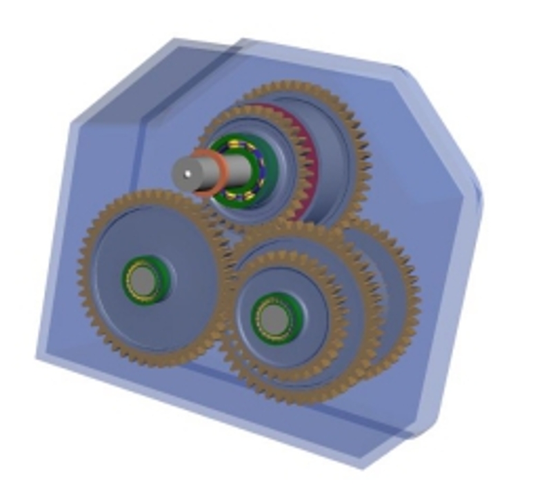
The new bevel gear – roller flat disk transmission combines the mechanisms of bevel gear and roller flat disk. The bevel gear part is responsible for changing the transmission ratio, while the roller flat disk part is in charge of smoothly transmitting torque. As shown in Figure 1, the power is first input to the bevel gear, and then transferred to the roller flat disk through meshing and rolling.
[Insert Figure 1: Structure of the New Bevel Gear – Roller Flat Disk Transmission]
2.2 Modeling of Bevel Gear Part
Let the input shaft speed of the bevel gear part be \(\omega_{in}\) and the output shaft speed be \(\omega_{out}\). Considering the influence of load changes on the transmission ratio, a load coefficient \(k_{L}\) is introduced. The transmission ratio i of the bevel gear can be expressed as: \(\begin{cases} \omega_{out}=\frac{\omega_{in}}{i}\\ i = \frac{N_{1}}{N_{2}}\cdot k_{L}(T_{out}) \end{cases}\) where \(k_{L}(T_{out})\) is a nonlinear function related to the output torque, representing the impact of load on the transmission ratio, and \(N_{1}\) and \(N_{2}\) are the numbers of teeth of the two bevel gears respectively.
2.3 Modeling of Roller Flat Disk Part
When the roller rolls on the flat disk, it is mainly affected by the frictional force \(F_{f}\). Assuming the friction coefficient between the roller and the flat disk is \(\mu\) and the normal pressure of the roller on the flat disk is \(F_{n}\), and considering that the rolling resistance moment \(M_{r}\) is related to factors such as the roller’s speed, acceleration, and material properties, a rolling resistance coefficient \(f_{r}\) is introduced. The rolling resistance moment \(M_{r}\) can be expressed as: \(M_{r}=f_{r}(v,\alpha,\mu,\rho,\cdots)\cdot F_{n}\cdot R\) where v represents the linear velocity of the roller, \(\alpha\) represents the angular acceleration of the roller, \(\rho\) represents the material density, and R represents the radius of the roller.
2.4 Integrated Dynamics Equation
By integrating the dynamics equations of the bevel gear and roller flat disk parts, the dynamics equation of the entire transmission can be obtained: \(T_{in}\cdot\frac{1}{i}-T_{out}=J_{out}\cdot\frac{d\omega_{out}}{dt}+M_{r}\) where \(J_{out}\) represents the moment of inertia of the output shaft, and \(T_{in}\) and \(T_{out}\) represent the input shaft torque and output shaft torque respectively. Table 2 summarizes the key parameters in the dynamics modeling.
| Parameter | Symbol | Description |
|---|---|---|
| Input shaft speed of bevel gear | \(\omega_{in}\) | The rotational speed of the input shaft of the bevel gear part |
| Output shaft speed of bevel gear | \(\omega_{out}\) | The rotational speed of the output shaft of the bevel gear part |
| Transmission ratio of bevel gear | i | The ratio of the input and output speeds of the bevel gear, affected by load |
| Load coefficient | \(k_{L}\) | A nonlinear function related to output torque, reflecting load impact on transmission ratio |
| Friction coefficient | \(\mu\) | The coefficient of friction between the roller and the flat disk |
| Normal pressure | \(F_{n}\) | The pressure exerted by the roller on the flat disk |
| Rolling resistance coefficient | \(f_{r}\) | A coefficient related to factors like speed, acceleration, and material properties |
| Rolling resistance moment | \(M_{r}\) | The moment that resists the rolling of the roller |
| Moment of inertia of output shaft | \(J_{out}\) | The inertia of the output shaft, affecting its rotational behavior |
| Input shaft torque | \(T_{in}\) | The torque input to the transmission |
| Output shaft torque | \(T_{out}\) | The torque output from the transmission |
3. Fuzzy Condition Setting
3.1 Selection of Input Variables
3.1.1 Error (e)
The error e is defined as the difference between the actual speed and the set speed, which reflects the current control deviation of the system. The formula is: \(e = e_{1}-e_{2}\) where \(e_{1}\) represents the measured value and \(e_{2}\) represents the set value.
3.1.2 Error Change Rate (ec)
The error change rate ec is the rate of change of the error over time, indicating the trend of the system deviation. The formula is: \(ec=\frac{e_{k}-e_{k – 1}}{\Delta t}\) where \(e_{k}\) represents the error at the current time point, \(e_{k-1}\) represents the error at the previous time point, and \(\Delta t\) represents the time interval.
3.2 Fuzzy Sets and Membership Functions
Fuzzy sets are defined for the error e and the error change rate ec. For example, the fuzzy sets can be {Negative Big, Negative Medium, Negative Small, Zero, Positive Small, Positive Medium, Positive Big}, denoted as \(\{NB, NM, NS, Z, PS, PM, PB\}\). Membership functions are used to describe the degree to which a value belongs to a certain fuzzy set. Figure 2 shows an example of triangular membership functions for error e.
[Insert Figure 2: Triangular Membership Functions for Error e]
3.3 Fuzzy Rule Base
Based on expert experience or the dynamic characteristics of the system, a fuzzy rule base is established. The rules are usually in the form of: “If e is X and ec is Y, then \(K_{p}\) is \(Z_{1}\), \(K_{i}\) is \(z_{2}\), \(K_{d}\) is \(Z_{3}\)”, where X, Y, \(Z_{1}\), \(z_{2}\), \(Z_{3}\) are elements of the fuzzy sets. Table 3 shows a sample of the fuzzy rule base.
| e | ec | \(K_{p}\) | \(K_{i}\) | \(K_{d}\) |
|---|---|---|---|---|
| NB | NB | NB | NB | PB |
| NB | NM | NB | NM | PB |
| \(\cdots\) | \(\cdots\) | \(\cdots\) | \(\cdots\) | \(\cdots\) |
3.4 Fuzzy Inference and Defuzzification
A fuzzy inference machine is used for fuzzy inference. According to the input e and ec, the adjustment values of the PID parameters are determined. After fuzzy inference, defuzzification is carried out to convert the fuzzy output into a precise value. One common defuzzification method is the weighted average method.
4. Design of Transmission Constant Speed Output Fuzzy PID Controller
4.1 Controller Structure
The output shaft speed deviation and its change rate are selected as the inputs of the fuzzy controller, and the output is set as the parameter adjustment amounts \(\Delta K_{p}\), \(\Delta K_{i}\), \(\Delta K_{d}\) of the controller. The structure of the designed fuzzy controller is shown in Figure 3.
[Insert Figure 3: Structure of the Fuzzy Controller]
4.2 Fuzzification of Inputs
Since the system deviation and deviation change rate are precise values, they need to be fuzzified and mapped to the fuzzy universe of discourse. Suppose the basic universe of discourse of the system deviation is \([-E, E]\), and the discrete fuzzy universe of discourse after fuzzification is \([-n, n]\), then the quantization factor \(k_{e}\) can be determined by the formula: \(k_{e}=\frac{n}{E}\) Similarly, for the deviation change rate, if its basic universe of discourse is \([-EC, EC]\) and the fuzzy universe of discourse is \([-m, m]\), the quantization factor is \(k_{ec}=\frac{m}{EC}\).
4.3 Adjustment of PID Parameters
In the constant speed output control of the roller flat disk transmission, the fuzzy PID control strategy can effectively improve the system’s adaptability and stability. The control parameters of the fuzzy controller are expressed as: \(\begin{cases} K_{p}=K_{p1}+\Delta K_{p}\\ K_{i}=K_{i1}+\Delta K_{i}\\ K_{d}=K_{d1}+\Delta K_{d} \end{cases}\) where \(K_{p1}\), \(K_{i1}\), \(K_{d1}\) are the initial parameters of the system. The impacts of PID parameters are as follows:
- Increasing the proportional coefficient \(K_{p}\) can speed up the system response, but if it is too large, it may lead to overshoot and oscillation.
- Increasing the integral coefficient \(K_{i}\) can enhance the system’s ability to eliminate steady – state errors, but an excessive value may slow down the system response or even make it unstable.
- Increasing the differential coefficient \(K_{d}\) can improve the system’s dynamic characteristics, reducing overshoot and oscillation, but it may increase the system’s sensitivity to noise.
5. Fuzzy PID Control Quantity Output
5.1 Design of Fuzzy Rules
Fuzzy subsets are used to evaluate the degree of deviation of the transmission’s constant speed. For example, it can be divided into {Negative Big, Negative Medium, Negative Small, Zero, Positive Small, Positive Medium, Positive Big}, and a fuzzy control rule table is constructed as shown in Table 4.
| e | ec | \(\Delta K_{p}\) | \(\Delta K_{i}\) | \(\Delta K_{d}\) |
|---|---|---|---|---|
| NB | NB | NB | NB | PB |
| NB | NM | NB | NM | PB |
| \(\cdots\) | \(\cdots\) | \(\cdots\) | \(\cdots\) | \(\cdots\) |
5.2 Defuzzification and Parameter Update
By combining the constructed fuzzy rules, the uncertainty of the system can be described using fuzzy variables. Then, through the weighted average method, the output of the fuzzy inference is converted into precise PID parameter adjustment amounts. The defuzzification output expressions of the PID parameter adjustment amounts are: \(\begin{cases} \Delta K_{p}=\frac{\sum_{i = 1}^{n}x_{i}\cdot\mu A_{p}(x_{i})}{\sum_{i = 1}^{n}\mu A_{p}(x_{i})}\\ \Delta K_{i}=\frac{\sum_{i = 1}^{n}x_{i}\cdot\mu A_{i}(x_{i})}{\sum_{i = 1}^{n}\mu A_{i}(x_{i})}\\ \Delta K_{d}=\frac{\sum_{i = 1}^{n}x_{i}\cdot\mu A_{d}(x_{i})}{\sum_{i = 1}^{n}\mu A_{d}(x_{i})} \end{cases}\) where \(A_{p}(x_{i})\), \(A_{i}(x_{i})\), \(A_{d}(x_{i})\) are the membership functions of the fuzzy sets for different PID parameter adjustment amounts. After obtaining the adjustment amounts, the PID controller parameters can be updated.
5.3 Calculation of Control Quantity
The control quantity \(u(t)\) is calculated using the updated PID parameters: \(u(t)=K_{p}(t)\cdot e(t)+K_{i}(t)\int_{0}^{t}e(t)dt + K_{d}(t)\frac{de(t)}{dt}\) where \(K_{p}(t)\), \(K_{i}(t)\), \(K_{d}(t)\) are the updated PID parameters, \(e(t)\) is the output shaft speed deviation, and \(u(t)\) is the control quantity. The control quantity \(u(t)\) is then converted into adjustment instructions for the input shaft speed or torque and sent to the transmission actuator to achieve constant control of the output shaft speed.
6. Simulation Experiments
6.1 Experiment Description
To prove the superiority of the proposed fuzzy PID control method for the constant speed output of the new bevel gear – roller flat disk transmission in practical control effects, two conventional transmission constant speed control methods are selected as comparison objects: the conventional transmission constant speed control method based on MPC and the conventional transmission constant speed control method based on the ant colony algorithm. A simulation experiment platform is constructed, and the three control methods are used to perform simulation speed output control on the same transmission model.
6.2 Experiment Object
The selected new bevel gear – roller flat disk transmission consists of a bevel gear transmission part and a roller flat disk stepless speed – change part. The bevel gear part can meet the requirements of high – speed transmission, and the roller flat disk part can achieve continuous speed change from low to high speed. The overall speed range is set from 500r/min to 3000r/min, which can meet the requirements of most automotive driving conditions. In ideal conditions, the transmission efficiency can reach over 95%. Table 5 shows the main parameters of the transmission for simulation modeling.
| Parameter | Configuration |
|---|---|
| Number of teeth of input bevel gear 1 | 50 |
| Number of teeth of bevel gear 3/4 | 55 |
| Number of teeth of bevel gear 5/6 | 65 |
| Number of teeth of input bevel gear 2 | 60 |
| Roller radius/mm | 50 |
| Flat disk radius/mm | 70 |
| Rolling resistance coefficient | 0.15 |
| Load coefficient | 0.01 |
| Number of added neurons | 5 |
| Maximum number of neurons | 100 |
| PID proportional coefficient | 0.1 |
| Integral time constant | 0.0004 |
| Differential time constant | 5.95 |
6.3 Comparison Results of Control Accuracy
The simulation speed output curves of the transmission obtained by different methods are shown in Figure 4. Under different load torque conditions, the proposed control method can achieve speed output control within a short adjustment time. The adjustment time of the system under 150/350N·m load torque conditions is within 4s. Table 6 shows the comparison results of overshoots under different control methods. It can be clearly seen that the proposed fuzzy PID control method has a significantly higher control accuracy than the two conventional control methods, with a lower maximum deviation value of the regulated quantity.
[Insert Figure 4: Output Speed Tracking Curves under Different Load Torque Conditions]
| Experimental Group Number | Design Method | Conventional Method A | Conventional Method B |
|---|---|---|---|
| 01 | 3.15 | 4.24 | 5.57 |
| 02 | 3.36 | 4.52 | 5.54 |
| \(\cdots\) | \(\cdots\) | \(\cdots\) | \(\cdots\) |
7. Conclusion
This paper has comprehensively studied the fuzzy PID control method for the constant speed output of the new bevel gear – roller flat disk transmission. By considering the nonlinear characteristics and uncertainties of the transmission system, a new control strategy has been successfully developed. The simulation experiments have verified that the fuzzy PID control method can effectively adapt to complex working environments, achieve constant speed output of the transmission, and improve the overall performance and stability of the transmission system. This research provides a new solution for the performance optimization of transmission systems and enriches the research content in the field of transmission system control. Future research can focus on further improving the real – time performance of the control method and applying it to more complex practical scenarios.