
I began this study from a practical manufacturing problem. High-production coal mines depend on reliable shearer equipment, and the drive gear used in the traction and haulage system is one of the most important wear-prone components. Because the drive gear transmits large torque, absorbs impact, and meshes with the haulage chain, it is difficult to replace underground. When gear cutting and the downstream finishing operations cannot meet demand, spare-part supply becomes unstable, and the mine may face costly downtime. My aim was therefore to examine the drive gear manufacturing process as a discrete-event dynamic system, build a Witness simulation model, identify bottlenecks in gear cutting and related operations, and propose an optimization plan that improves throughput without uncontrolled capital expenditure.
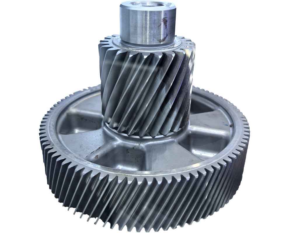
I treated the production system as a network of machines, buffers, labor resources, and part flows. The system is neither purely continuous nor purely deterministic. It is a discrete-event system because the state changes when a part arrives, a machine starts or finishes gear cutting, a batch heat-treatment cycle ends, a buffer reaches capacity, or a worker performs an adjustment. I used Witness because it supports event scheduling, graphical animation, resource modeling, rule-based input and output logic, and statistical reporting. The model allowed me to compare the existing gear cutting process with several improvement scenarios before making changes on the shop floor.
| Research stage | Practical question | Method used | Output |
|---|---|---|---|
| Problem definition | Why is drive gear supply late? | Field observation and process mapping | Bottleneck hypotheses |
| System abstraction | What type of system is the gear cutting line? | Discrete-event dynamic system analysis | Entity, resource, and event structure |
| Data collection | What are the operation times and machine counts? | Routing sheets and time studies | Input distributions and cycle times |
| Model construction | How can the process be represented in Witness? | Machine, buffer, labor, part, variable elements | Simulation model |
| Validation | Does the model represent real gear cutting flow? | Trace checks and logical verification | Accepted baseline model |
| Optimization | Which changes improve throughput? | Quantity, time, and combined scenarios | Preferred configuration |
I defined the gear cutting process route from forging preparation to final fitting. The main operations include rough turning, stress relief, semi-finish turning, wire-cut electrical discharge machining for rough gear cutting, hobbing for semi-finish gear cutting, fitting, carburizing, semi-finish turning, quenching, finish turning, external grinding, wire-cut internal spline machining, profile grinding for final gear cutting, and final fitting. The gear cutting steps are not isolated. They interact with heat treatment, turning, grinding, and inspection. This interaction makes the gear cutting lead time long and variable.
| Sequence | Operation content | Machine group | Time per piece or batch | Available machines |
|---|---|---|---|---|
| 05 | Rough turning of surfaces | Turning group | 11.00 h | 20 |
| 10 | Stress relief heat treatment | Heat treatment group | 12.00 h | 9 |
| 15 | Semi-finish turning | Turning group | 5.50 h | 20 |
| 20 | Wire-cut rough gear cutting | Wire EDM group | 75.42 h | 14 |
| 25 | Hobbing semi-finish gear cutting | Hobbing group | 31.00 h | 2 |
| 30 | Fitting and tooth edge chamfering | Fitting group | 1.00 h | 2 |
| 35 | Carburizing of tooth surfaces | Heat treatment group | 110.00 h | 5 |
| 40 | Semi-finish turning of outer surfaces | Turning group | 4.50 h | 20 |
| 45 | Overall quenching | Heat treatment group | 16.00 h | 2 |
| 50 | Finish turning with grinding allowance | Turning group | 2.00 h | 20 |
| 55 | External surface grinding | Grinding group | 5.00 h | 3 |
| 60 | Internal surface finish turning | Turning group | 2.00 h | 20 |
| 65 | Wire-cut internal spline | Wire EDM group | 27.50 h | 14 |
| 70 | Profile gear cutting and grinding | Profile grinding group | 9.25 h | 2 |
| 75 | Deburring | Fitting group | 1.00 h | 2 |
I grouped the detailed routing into seven resource groups to make the simulation manageable: turning, wire EDM, hobbing, grinding, profile grinding, fitting, and heat treatment. I converted all times to minutes for the model. The total nominal processing content per drive gear is large, and the gear cutting operations alone consume a major share of the total cycle time. Wire EDM rough gear cutting, hobbing semi-finish gear cutting, and profile grinding final gear cutting are especially important because they determine both geometry and quality.
| Resource group | Number of machines | Total processing time per gear in minutes | Role in gear cutting |
|---|---|---|---|
| Turning group | 20 | 1500 | Preparation and finishing of datum surfaces |
| Wire EDM group | 14 | 6175 | Rough gear cutting and internal spline cutting |
| Hobbing group | 2 | 1860 | Semi-finish gear cutting |
| Grinding group | 3 | 270 | External surface preparation |
| Profile grinding group | 2 | 555 | Final gear cutting and tooth profile finishing |
| Fitting group | 2 | 120 | Chamfering and deburring |
| Heat treatment group | 9 | 8280 | Stress relief, carburizing, and quenching |
I represent the gear cutting system with formal variables. Let \(M_i(t)\) be the state of machine group \(i\) at time \(t\), where the state may be busy, idle, blocked, or under repair. Let \(N(t)\) be the number of parts in the system. Let \(E(t)\) be the set of active events. The general discrete-event state transition can be written as
$$X(t+\Delta t)=F\bigl(X(t),E(t),U(t)\bigr),$$
where \(X(t)\) is the system state, \(E(t)\) is the event set, and \(U(t)\) is the control or decision input. In my model, the events include part arrival, machine loading, machine unloading, batch heat-treatment completion, worker adjustment, and buffer blockage.
The event scheduling logic follows the earliest-event rule. If \(t_{now}\) is the current simulation time, the next event time is
$$t_{next}=\min\{t_e : t_e>t_{now},\ e\in E_{active}\}.$$
This is one reason I selected Witness. It manages the event calendar automatically and allows me to focus on the gear cutting logic rather than on low-level clock control.
I used several performance measures to judge the gear cutting process. Utilization of machine group \(i\) is
$$U_i=\frac{1}{T}\int_0^T \mathbf{1}\{M_i(t)=\text{busy}\}\,dt.$$
Throughput is
$$TP=\frac{N_{shipped}}{T}.$$
The average work in process is
$$\overline{WIP}=\frac{1}{T}\int_0^T N(t)\,dt.$$
Little’s law connects flow, time, and inventory:
$$\overline{WIP}=\lambda \overline{W},$$
where \(\lambda\) is the arrival or completion rate and \(\overline{W}\) is the average time a part spends in the system. I used this relationship to interpret the long average stay time of drive gears.
For a multi-machine group, I estimated the load intensity as
$$\rho_i=\frac{\lambda_i}{m_i\mu_i},$$
where \(m_i\) is the number of machines in group \(i\), \(\lambda_i\) is the arrival rate to that group, and \(\mu_i\) is the service rate of one machine. If \(\rho_i\) approaches or exceeds one, a queue grows and the group becomes a bottleneck. I also defined the bottleneck index as
$$B=\arg\max_i U_i.$$
For batch operations such as carburizing, the effective cycle time is not simply the sum of individual processing times. I used
$$CT_{batch}=\max\{t_{load},t_{cycle},t_{unload}\}+t_{wait},$$
where \(t_{load}\) is loading time, \(t_{cycle}\) is the furnace cycle, \(t_{unload}\) is unloading time, and \(t_{wait}\) is waiting before or after the batch operation. This formula helped me explain why heat treatment creates long waiting periods even when furnace utilization appears moderate.
I built the model in Witness using four main element classes: parts, machines, buffers, and labor. I also used variables and time-series elements to track output and work in process. The part element represents the drive gear forging as it moves through the process. Machine elements represent the turning group, wire EDM group, hobbing group, grinding group, profile grinding group, fitting group, and heat treatment group. Buffer elements represent the queues before major gear cutting operations. Labor elements represent shared operators and setup personnel. Variables record the number of shipped parts and the amount of work in process.
| Witness element | Type | Quantity | Function in the gear cutting model |
|---|---|---|---|
| Drive gear part | Part | 1 type | Entity moving through the gear cutting route |
| Heat treatment group | Machine | 1 logical group | Stress relief, carburizing, and quenching |
| Turning group | Machine | 4 logical machines in the simplified model | Rough, semi-finish, and finish turning |
| Wire EDM group | Machine | 4 logical machines in the simplified model | Rough gear cutting and internal spline cutting |
| Hobbing group | Machine | 2 logical machines | Semi-finish gear cutting |
| Grinding group | Machine | 3 logical machines | External grinding |
| Profile grinding group | Machine | 2 logical machines | Final gear cutting and tooth profile finishing |
| Fitting group | Machine | 1 logical group | Chamfering and deburring |
| Input buffers | Buffer | 5 | Queue before selected gear cutting and finishing operations |
| Labor | Labor | Shared resource | Setup, adjustment, and manual operations |
| Shipped count | Variable | 1 | Tracks completed drive gears |
| Time series | Time series | 1 | Displays work in process over time |
I used single-machine logic for most operations and batch-machine logic for heat treatment. The input rules were written with pull and push conditions. For example, a turning machine pulls a part only when the downstream wire EDM buffer has space. The wire EDM group pulls from its buffer when a machine is free. The hobbing group pulls from the wire EDM buffer when a hobbing machine is available. The heat treatment group accumulates a batch and processes it as a batch. This rule structure allows the model to reproduce blocking, starvation, and queue growth.
I validated the model in three ways. First, I checked the logical sequence against the process route to confirm that no gear cutting operation was omitted. Second, I traced individual parts and verified that event times matched the expected cycle times. Third, I compared the model output with observed shop-floor behavior. For example, when the simulation clock reached the first completion point, the part had moved into the wire EDM buffer, and the turning group had completed its first operation. The trace confirmed that the gear cutting sequence behaved as intended.
| Validation item | Check performed | Result |
|---|---|---|
| Route logic | Compare model sequence with routing sheet | Matched |
| Event timing | Trace first part through turning and wire EDM | Matched expected timing |
| Buffer behavior | Observe queue growth before gear cutting | Consistent with shop floor |
| Machine states | Check busy, idle, and blocked states | Reasonable |
| Output level | Compare monthly output with historical supply | Within observed range |
After validation, I ran the baseline model for a simulated month. I defined one month as thirty days of continuous operation with eight working hours per day, giving a simulation horizon of 14400 minutes. Because the model contains random variation, I used independent replications. For replication \(r\), let \(Y_r\) be the output. The sample mean is
$$\bar{Y}=\frac{1}{R}\sum_{r=1}^{R}Y_r,$$
and the standard error is
$$s_{\bar{Y}}=\frac{s}{\sqrt{R}}.$$
I used these statistics to compare scenarios. The baseline model produced approximately 43 drive gears per month. The average work in process was about 20.33 parts, and the average time in the system was about 157.52 hours. The largest delays occurred before and within the wire EDM and hobbing stages. The wire EDM group carried a high load because it performed both rough gear cutting and internal spline cutting. The hobbing group had only two machines and therefore had limited capacity for semi-finish gear cutting. The profile grinding group also became important because final gear cutting quality depends on it.
| Baseline performance measure | Value | Interpretation |
|---|---|---|
| Simulation horizon | 14400 min | One month, 8 hours per day |
| Monthly output | 43 gears | Baseline capacity |
| Average work in process | 20.33 parts | Large queue content |
| Average time in system | 157.52 h | Long manufacturing lead time |
| Main bottleneck indicators | Wire EDM and hobbing | Gear cutting capacity limits flow |
| Secondary constraint | Profile grinding | Final gear cutting capacity |
I then tested three families of optimization. The first family changed quantity factors, meaning the number of machines in selected groups. The second family changed time factors, meaning cycle times and adjustment times. The third family combined quantity and time changes. I evaluated each scenario with the same simulation horizon and multiple independent replications. The objective function was
$$\max_{m,t} TP(m,t)$$
subject to
$$m_i \le m_i^{max},\qquad t_{ij} \ge t_{ij}^{min},\qquad U_i \le U_i^{max},\qquad C(m,t)\le C_{budget},$$
where \(m\) is the machine quantity vector, \(t\) is the time vector, \(C\) is cost, and \(U_i^{max}\) is an acceptable upper utilization limit. I did not want to increase every machine group, because many machines are expensive computer numerical control assets. I wanted a balanced configuration that removes the gear cutting bottleneck without creating a new one.
| Scenario family | Decision variables | Expected effect | Risk |
|---|---|---|---|
| Quantity change | Number of machines in wire EDM, hobbing, and related groups | Increase capacity directly | Higher capital cost and possible new bottleneck |
| Time change | Cycle time, setup time, and adjustment time | Improve efficiency without new machines | Limited by process physics and quality requirements |
| Combined change | Machine quantity and time together | Balance load and raise throughput | Requires careful scheduling and validation |
In the first quantity scenario, I increased selected capacities to relieve the gear cutting bottleneck. I increased the wire EDM capacity and adjusted the turning group representation, then ran seven independent replications. The monthly output rose from 43 to about 51 gears. However, the hobbing group reached a very high utilization, above 96 percent. This meant that the gear cutting flow had shifted from wire EDM to hobbing. The system had improved, but it was not yet balanced.
| Machine group | Replication 1 | Replication 2 | Replication 3 | Replication 4 | Replication 5 | Replication 6 | Replication 7 | Average |
|---|---|---|---|---|---|---|---|---|
| Turning | 66.21 | 66.09 | 66.22 | 66.14 | 66.13 | 66.18 | 66.14 | 66.16 |
| Wire EDM | 66.35 | 66.26 | 66.43 | 66.29 | 66.32 | 66.40 | 66.23 | 66.33 |
| Hobbing | 96.88 | 96.81 | 96.94 | 96.83 | 96.85 | 96.90 | 96.79 | 96.86 |
| Grinding | 76.71 | 76.71 | 76.74 | 76.75 | 76.70 | 76.65 | 76.76 | 76.72 |
| Profile grinding | 9.85 | 9.85 | 9.84 | 9.87 | 9.85 | 9.86 | 9.85 | 9.86 |
In the second quantity scenario, I increased the hobbing group from two machines to three machines. This directly addressed the new bottleneck. The monthly output increased to about 58 gears. The hobbing utilization dropped to about 55 percent, while profile grinding rose to about 84.70 percent. This result showed that the gear cutting system had been improved further, but the final gear cutting resource had become the next constraint. The system was moving toward a more balanced state.
| Machine group | Average utilization in scenario 1 | Average utilization in scenario 2 | Change |
|---|---|---|---|
| Turning | 66.16 | 74.64 | Increased |
| Wire EDM | 66.33 | 75.75 | Increased |
| Hobbing | 96.86 | 55.01 | Decreased sharply |
| Grinding | 76.72 | 55.39 | Decreased |
| Profile grinding | 9.86 | 84.70 | Increased sharply |
In the time-factor scenarios, I reduced setup and adjustment times where advanced equipment allowed faster processing. I also adjusted the process times for selected gear cutting operations. The heat treatment times were held nearly constant because thermal cycles cannot be shortened without affecting metallurgical quality. The result was only a modest output improvement. The utilization of some groups changed, but the system still had a bottleneck. This confirmed that time reduction alone could not solve the gear cutting capacity problem, especially when the bottleneck is created by a small number of specialized machines.
| Machine group | Average utilization after time optimization | Observation |
|---|---|---|
| Turning | 98.28 | Very high load |
| Wire EDM | 80.31 | Still a major constraint |
| Hobbing | 63.93 | Improved but not balanced |
| Grinding | 8.20 | Low utilization |
| Profile grinding | 98.28 | Very high load |
In the combined scenario, I changed both quantity and time factors. I used advanced equipment capability to shorten selected cycle times and increased capacity in the most restrictive gear cutting groups. I ran seven independent replications with the same 14400-minute horizon. The combined scenario produced about 62 gears per month. Profile grinding remained the highest utilized group at about 84.70 percent, while hobbing, grinding, and other groups were below 70 percent. The line was more balanced, and the output gain was larger than in the single-factor scenarios.
| Machine group | Replication 1 | Replication 2 | Replication 3 | Replication 4 | Replication 5 | Replication 6 | Replication 7 | Average |
|---|---|---|---|---|---|---|---|---|
| Turning | 67.57 | 67.61 | 67.46 | 67.53 | 67.54 | 67.50 | 67.58 | 67.54 |
| Wire EDM | 66.48 | 66.54 | 66.44 | 66.41 | 66.52 | 66.43 | 66.47 | 66.47 |
| Hobbing | 39.39 | 39.43 | 39.36 | 39.34 | 39.37 | 39.35 | 39.33 | 39.37 |
| Grinding | 39.35 | 39.33 | 39.35 | 39.37 | 39.31 | 39.34 | 39.38 | 39.35 |
| Profile grinding | 84.71 | 84.76 | 84.71 | 84.69 | 84.67 | 84.65 | 84.72 | 84.70 |
I compared the scenarios with two criteria: monthly output and utilization balance. The baseline output was 43 gears per month. The first quantity scenario reached about 51 gears. The second quantity scenario reached about 58 gears. The combined scenario reached about 62 gears. Therefore, the combined scenario improved gear cutting throughput by approximately
$$\eta=\frac{TP_{opt}-TP_{base}}{TP_{base}}\times 100\% =\frac{62-43}{43}\times 100\% \approx 44.2\%.$$
If I use the conservative optimized range of 55 to 60 gears per month, the improvement is
$$\eta_{min}=\frac{55-43}{43}\times 100\% \approx 27.9\%,$$
$$\eta_{max}=\frac{60-43}{43}\times 100\% \approx 39.5\%.$$
This range is consistent with the observed conclusion that gear cutting efficiency improved by about 35 percent. The exact value depends on random variation, operator availability, and the actual machine configuration.
| Scenario | Monthly output | Main bottleneck | Balance assessment |
|---|---|---|---|
| Baseline | 43 gears | Wire EDM and hobbing | Poor balance |
| Quantity scenario 1 | 51 gears | Hobbing | Improved but shifted bottleneck |
| Quantity scenario 2 | 58 gears | Profile grinding | Better balance |
| Time scenario | Modest increase | Turning and profile grinding | Limited benefit |
| Combined scenario | 62 gears | Profile grinding | Best balance and throughput |
The gear cutting simulation also showed that equipment utilization alone is not a sufficient decision criterion. A group with high utilization may be a bottleneck, but adding capacity there can shift the bottleneck elsewhere. For example, increasing wire EDM capacity reduced the wire EDM queue but exposed the hobbing limitation. Increasing hobbing capacity then exposed profile grinding. This is the classic shifting-bottleneck behavior of a discrete manufacturing system. The correct optimization is therefore not simply to maximize every machine group. It is to balance the gear cutting chain so that no single group starves the rest of the system.
I used independent replications because a single run can be misleading. The confidence interval for the mean output is
$$\bar{Y}\pm t_{R-1,1-\alpha/2}\frac{s}{\sqrt{R}}.$$
With seven replications, I obtained a reasonable estimate of the expected performance. The variation across replications was small for machine utilization, which suggests that the model logic was stable. The variation was larger for work in process and lead time because queues amplify random events. This is especially true before gear cutting operations, where a small delay in hobbing or wire EDM can create a long queue.
I also examined the relationship between setup time, adjustment time, and system output. Let \(t_{setup}\) be setup time and \(t_{adj}\) be adjustment time. The effective processing time for a gear cutting operation can be approximated as
$$t_{eff}=t_{process}+t_{setup}+t_{adj}+t_{wait}.$$
The sensitivity of throughput to these components is not equal. In my experiments, the adjustment and setup time of highly utilized gear cutting machines had a larger effect than the adjustment time of lightly utilized machines. This is intuitive: if a machine is not a constraint, reducing its setup time does not increase system throughput. If a machine is a constraint, reducing its setup time increases capacity. This principle guided my optimization priority.
The labor resource also influenced the gear cutting process. Shared operators perform setup, adjustment, and inspection. If a machine finishes processing but no operator is available, the machine may remain blocked. The effective capacity of a machine group with labor constraints can be written as
$$C_i=m_i\cdot \frac{T}{t_{cycle,i}}\cdot A_i\cdot L_i,$$
where \(A_i\) is machine availability and \(L_i\) is the probability that the required labor is available. When \(L_i\) is low, the actual capacity is lower than the nominal machine capacity. In the baseline model, the wire EDM group had significant waiting for adjustment, which increased the effective gear cutting cycle time. This supported the conclusion that both hardware capacity and labor allocation matter.
Heat treatment is another critical part of gear cutting because it changes material properties and creates long batch delays. The carburizing and quenching operations cannot be treated as simple single-piece operations. A batch furnace processes several gears at once, and the cycle time is dominated by thermal diffusion and soaking. If the batch is not full, capacity is wasted. If the batch is too large, downstream gear cutting and grinding may be starved or flooded. I therefore modeled heat treatment with batch logic and examined how it interacts with gear cutting. The results showed that heat treatment is not always the highest-utilization resource, but it creates long waiting times because of batching and transfer. This waiting time contributes to the average 157.52 hours in the system.
From a management perspective, the simulation provides a decision-support tool. It allows me to test a machine purchase, a process improvement, or a scheduling change before committing capital. The model can answer questions such as:
What happens if I add one hobbing machine? How much does monthly gear cutting output increase? Does the bottleneck move to profile grinding? What is the effect of reducing wire EDM adjustment time? How many operators are needed to keep the gear cutting cells running? What is the trade-off between capital cost and throughput gain? These questions are difficult to answer with spreadsheet calculations alone because they involve queues, random failures, batch operations, and shared resources.
| Decision question | Simulation evidence | Recommendation |
|---|---|---|
| Should wire EDM capacity be increased first? | Baseline queue before wire EDM is long | Yes, but only as part of a balanced plan |
| Should hobbing capacity be increased? | After wire EDM improvement, hobbing utilization exceeds 96 percent | Yes, to prevent a new bottleneck |
| Should profile grinding capacity be increased? | After hobbing improvement, profile grinding becomes the highest utilized group | Monitor and plan capacity when demand rises |
| Can time reduction alone solve the problem? | Time-only scenarios provide only modest gains | No, combine time reduction with capacity balancing |
| Is the combined scenario preferred? | Highest output and better balance | Yes, use as the main improvement direction |
I also examined the cost side. Let \(\Delta C\) be the additional cost of added machines and process improvements, and let \(\Delta R\) be the additional revenue from higher gear cutting output. The net benefit is
$$NB=\Delta R-\Delta C.$$
A positive net benefit indicates that the improvement is economically justified. In my study, the combined scenario offered the best balance because it avoided excessive machine additions while still raising output. Adding too many machines would increase cost and reduce utilization, which is not desirable. The simulation showed that a moderate capacity increase in the right places is more effective than a large across-the-board increase.
The results also have implications for gear cutting scheduling. When the hobbing group is a bottleneck, the schedule should protect hobbing capacity by ensuring that it never starves. When profile grinding is the bottleneck, the schedule should ensure that finished gear cutting operations are paced to match profile grinding. When wire EDM is the bottleneck, reducing setup and adjustment time is valuable. This is a dynamic priority rule: the bottleneck should receive the highest scheduling attention. In mathematical form, the scheduling priority can be written as
$$P_i=\alpha U_i+\beta Q_i+\gamma D_i,$$
where \(U_i\) is utilization, \(Q_i\) is queue length, \(D_i\) is downstream demand urgency, and \(\alpha,\beta,\gamma\) are weights. The bottleneck group has the largest \(P_i\) and should be protected from starvation and blockage.
I found that the gear cutting process is sensitive to initial conditions and random disturbances. A machine failure during a critical gear cutting operation can create a large queue because the downstream operations continue to demand parts. A batch heat-treatment delay can starve hobbing, and a hobbing delay can starve profile grinding. This confirms that the system is a discrete-event dynamic system with nonlinear interactions. The simulation model is therefore more informative than a static capacity calculation.
In terms of model limitations, I simplified some operations into logical groups. I did not model every individual machine, every tool change, or every maintenance event. I also assumed that the process times remain stable within a scenario. In reality, tool wear, operator skill, and material variability can change gear cutting times. Future work could extend the model by adding tool life, preventive maintenance, and real-time data collection. It could also connect the simulation to a scheduling system so that the model can support daily dispatching.
Despite these limitations, the model provides useful conclusions. The baseline monthly capacity was about 43 drive gears. The optimized combined scenario reached about 55 to 62 drive gears per month. The gear cutting efficiency improved by approximately 35 percent when using the conservative range. The main bottleneck moved from wire EDM and hobbing toward profile grinding. The system became more balanced, and the average utilization of non-bottleneck groups decreased. This means that the improvement did not simply push the problem to another part of the line without considering the whole system. Instead, it created a more stable gear cutting flow.
| Performance indicator | Baseline | Optimized | Improvement |
|---|---|---|---|
| Monthly output | 43 gears | 55 to 62 gears | About 28 to 44 percent |
| Gear cutting efficiency | Reference level | Improved | About 35 percent |
| Main bottleneck | Wire EDM and hobbing | Profile grinding | Bottleneck shifted and reduced |
| Average work in process | 20.33 parts | Better controlled | Queue pressure reduced |
| Average time in system | 157.52 h | Reduced in optimized runs | Lead time improved |
I conclude that Witness is an effective tool for gear cutting process simulation. It allowed me to convert a complex manufacturing problem into a transparent model with parts, machines, buffers, labor, and rules. It also allowed me to test optimization scenarios without disrupting production. The model can be used for production planning, capacity expansion, scheduling policy, and continuous improvement. The most important lesson is that gear cutting capacity should be managed as a chain, not as a set of isolated operations. Improving one gear cutting operation without considering the next can shift the bottleneck and reduce the benefit of the investment.
For future application, I recommend a periodic simulation review. As demand changes, as new gear cutting equipment is installed, and as product mix changes, the model should be updated. The updated model can then be used to evaluate new scenarios. This creates a closed-loop decision process: observe the real system, update the model, simulate alternatives, implement the best option, and measure the result. This loop supports continuous improvement and helps the enterprise respond faster to spare-part demand.
In summary, my study shows that a drive gear manufacturing system can be modeled as a discrete-event dynamic system and optimized with Witness. The baseline gear cutting process was constrained by wire EDM and hobbing capacity. Increasing capacity in a targeted way improved monthly output, but the system required a combined quantity and time optimization to avoid creating a new bottleneck. The combined scenario produced the best result, raising monthly output from 43 to approximately 55 to 62 gears and improving gear cutting efficiency by about 35 percent. The model provides a practical basis for production management, process optimization, and system analysis.