
I study high-speed dry gear hobbing as a green gear manufacturing process that can reduce pollution, shorten the process chain, and improve productivity. In my research, I focus on the geometric topography of the tooth surface finished by gear hobbing and on the normal deviation between the actual generated surface and the theoretical tooth surface. I combine spatial kinematic modeling, numerical simulation, sensitivity analysis, machine-learning surrogate modeling, Bayesian optimization, and virtual numerical-control machining to understand how hob design parameters and process parameters influence the finished gear tooth surface. The central aim is to find parameter combinations that reduce the normal deviation of the generated tooth surface during gear hobbing and to provide a reliable decision tool for high-quality gear manufacturing.
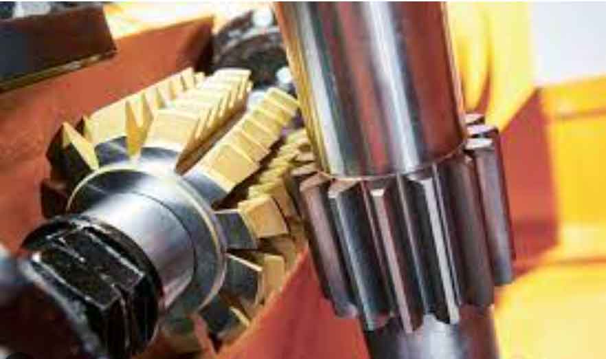
Gear hobbing is one of the most efficient and economical methods for manufacturing external cylindrical gears. In high-speed dry gear hobbing, no cutting fluid is used, so the process offers environmental benefits and high material-removal rates. However, because the hob removes material with a limited number of interrupted cutting edges, the actual tooth surface is not identical to the theoretical involute surface. The generated surface deviates from the theoretical surface in the normal direction, producing periodic textures that resemble fish scales. These deviations can increase vibration, friction, and noise in gear transmission. Therefore, I model the gear hobbing process from its spatial geometry and then optimize the key parameters that control the normal deviation of the generated tooth surface.
Kinematic and Geometric Model of Gear Hobbing
I treat gear hobbing as a spatial meshing process between a hob and a gear workpiece. The hob and the gear rotate according to a strict transmission ratio, and the gear or hob also moves along the axial direction to generate the full tooth width. The basic motion relationship is defined by the shaft angle, the center distance, and the transmission ratio. The shaft angle is
$$ \Sigma = \beta – \lambda $$
where \(\beta\) is the gear helix angle and \(\lambda\) is the hob lead angle. The center distance is
$$ a = r_h + r_g $$
where \(r_h\) is the hob pitch radius and \(r_g\) is the gear pitch radius. For the rotational motion, I use
$$ \phi_g = \frac{Z_h}{Z_g}\phi_h + \frac{\zeta}{p_g} $$
where \(\phi_g\) and \(\phi_h\) are the rotation angles of the gear and hob, \(Z_g\) and \(Z_h\) are the tooth number of the gear and the number of hob starts, \(\zeta\) is the axial feed displacement, and \(p_g\) is the gear helical parameter. For axial feed in gear hobbing, the feed displacement can be written as
$$ \zeta(\phi_h) = \zeta_0 \pm \frac{n f \phi_h}{2\pi} $$
where \(f\) is the feed per gear revolution, \(n\) is the number of revolutions, and the sign depends on climb hobbing or conventional hobbing. These relations form the kinematic foundation of the gear hobbing simulation.
I use homogeneous coordinate transformations to describe the relative motion between the hob and the gear. A general rotation matrix about the \(x\), \(y\), and \(z\) axes can be written as
$$ \mathbf{R}_x(\theta)=
\begin{bmatrix}
1 & 0 & 0 & 0\\
0 & \cos\theta & -\sin\theta & 0\\
0 & \sin\theta & \cos\theta & 0\\
0 & 0 & 0 & 1
\end{bmatrix},
\quad
\mathbf{R}_y(\theta)=
\begin{bmatrix}
\cos\theta & 0 & \sin\theta & 0\\
0 & 1 & 0 & 0\\
-\sin\theta & 0 & \cos\theta & 0\\
0 & 0 & 0 & 1
\end{bmatrix},
$$
$$
\mathbf{R}_z(\theta)=
\begin{bmatrix}
\cos\theta & -\sin\theta & 0 & 0\\
\sin\theta & \cos\theta & 0 & 0\\
0 & 0 & 1 & 0\\
0 & 0 & 0 & 1
\end{bmatrix}.
$$
The translation matrices are
$$ \mathbf{T}_x(l)=
\begin{bmatrix}
1 & 0 & 0 & l\\
0 & 1 & 0 & 0\\
0 & 0 & 1 & 0\\
0 & 0 & 0 & 1
\end{bmatrix},
\quad
\mathbf{T}_y(l)=
\begin{bmatrix}
1 & 0 & 0 & 0\\
0 & 1 & 0 & l\\
0 & 0 & 1 & 0\\
0 & 0 & 0 & 1
\end{bmatrix},
\quad
\mathbf{T}_z(l)=
\begin{bmatrix}
1 & 0 & 0 & 0\\
0 & 1 & 0 & 0\\
0 & 0 & 1 & l\\
0 & 0 & 0 & 1
\end{bmatrix}.
$$
In gear hobbing, the hob and gear coordinate systems are connected by a sequence of rotations and translations. I define the hob coordinate system \(S_h(x_h,y_h,z_h)\) and the gear coordinate system \(S_g(x_g,y_g,z_g)\). The hob rotates about its own axis, while the gear rotates about its axis and translates along the gear axis. The transformation from the hob to the gear can be expressed as
$$ \mathbf{r}_g(u,\theta,\phi_h,\zeta)=
\mathbf{M}_{g-go}\mathbf{M}_{go-ho}\mathbf{M}_{ho-h}\mathbf{r}_h(u,\theta). $$
Here, \(\mathbf{M}_{ho-h}\) maps the hob body coordinates into the hob observer coordinates, \(\mathbf{M}_{go-ho}\) maps the hob observer coordinates into the gear observer coordinates, and \(\mathbf{M}_{g-go}\) maps the gear observer coordinates into the gear body coordinates. This transformation is the core of my gear hobbing surface-generation model.
Hob Geometry and Cutting-Edge Parameterization
I construct the hob from a standard basic rack profile. The normal rack profile is composed of several straight and circular segments. The position vector of the normal rack profile is
$$ \mathbf{r}_n(u)=[x_n(u),0,z_n(u),1]^T. $$
The normal rack profile moves along the tooth-width direction and rotates by the lead angle \(\lambda\). The transformation from the normal rack coordinate system to the rack coordinate system is
$$ \mathbf{r}_r(u,v)=\mathbf{M}_{rn}\mathbf{r}_n(u), $$
where
$$ \mathbf{M}_{rn}=
\begin{bmatrix}
1 & 0 & 0 & 0\\
0 & \cos\lambda & -\sin\lambda & v\cos\lambda\\
0 & \sin\lambda & \cos\lambda & v\sin\lambda\\
0 & 0 & 0 & 1
\end{bmatrix}. $$
The basic rack profile segments can be summarized as follows.
| Segment | Parameter expression | Parameter range |
|---|---|---|
| AB | \(x_{AB}(u)=-h_{aP},\; z_{AB}(u)=u\) | \(-p_n/2 \le u \le -p_n/2 + h_{aP}\tan\alpha_n\) |
| BC | \(x_{BC}(u)=u+(p_n/4)\cot\alpha_n,\; z_{BC}(u)=u\) | \(z_B \le u \le z_C\) |
| CD | \(x_{CD}(u)=h_{fP}-\rho_{fP}+\sqrt{\rho_{fP}^2-(u-z_D)^2},\; z_{CD}(u)=u\) | \(z_C \le u \le z_D\) |
| DE | \(x_{DE}(u)=h_{fP},\; z_{DE}(u)=u\) | \(z_D \le u \le z_E\) |
| EF | \(x_{EF}(u)=h_{fP}-\rho_{fP}+\sqrt{\rho_{fP}^2-(u-z_F)^2},\; z_{EF}(u)=u\) | \(z_E \le u \le z_F\) |
| FG | \(x_{FG}(u)=u-(p_n/4)\cot\alpha_n,\; z_{FG}(u)=u\) | \(z_F \le u \le z_G\) |
| GH | \(x_{GH}(u)=-h_{aP},\; z_{GH}(u)=u\) | \(z_G \le u \le p_n/2\) |
The basic rack profile is then wrapped onto the hob to form the hob generating surface. I apply the meshing equation between the rack and the hob worm:
$$ f_w(u,v,\phi_w)=
\left(
\frac{\partial \mathbf{r}_w}{\partial u}
\times
\frac{\partial \mathbf{r}_w}{\partial v}
\right)
\cdot
\frac{\partial \mathbf{r}_w}{\partial \phi_w}=0. $$
Solving this equation gives the relation \(v=v(u,\phi_w)\), and the hob worm surface can be written as \(\mathbf{r}_w(u,\phi_w)\). The cutting edges are formed by the intersection of the hob worm surface and the front face of the hob. The front face introduces an additional constraint:
$$ \frac{y_w}{x_w}=-\tan\gamma, $$
where \(\gamma\) is the rake angle. The cutting edge is therefore parameterized by a single parameter \(u\). I write the cutting edge as
$$ \mathbf{r}_E(u)=[x_E(u),y_E(u),z_E(u),1]^T. $$
By sweeping the cutting edge along the hob helix, I obtain
$$ \mathbf{r}_h(u,\theta)=\mathbf{M}_{hE}\mathbf{r}_E(u), $$
where \(\theta\) is the rotation angle of the helical sweep and \(\mathbf{M}_{hE}\) is the helical transformation matrix. This parameterization allows me to place every cutting edge in the hob coordinate system and to simulate the cutting action during gear hobbing.
Generation of the Tooth Surface and Normal Deviation
The actual tooth surface in gear hobbing is generated by the envelope of the cutting edges. Because the hob has a finite number of flutes and because the feed motion is discrete, the actual surface is not a perfect involute surface. It is instead the envelope of a discrete family of cutting-edge trajectories. The surface family is
$$ \mathbf{r}_g(u,\theta,\phi_h,\zeta)=
\mathbf{M}_{g-go}\mathbf{M}_{go-ho}\mathbf{M}_{ho-h}\mathbf{r}_h(u,\theta). $$
I impose the meshing condition in two independent motion directions:
$$ f_h(u,\theta,\phi_h,\zeta)=
\left(
\frac{\partial \mathbf{r}_g}{\partial u}
\times
\frac{\partial \mathbf{r}_g}{\partial \theta}
\right)
\cdot
\frac{\partial \mathbf{r}_g}{\partial \phi_h}=0, $$
$$ f_\zeta(u,\theta,\phi_h,\zeta)=
\left(
\frac{\partial \mathbf{r}_g}{\partial u}
\times
\frac{\partial \mathbf{r}_g}{\partial \theta}
\right)
\cdot
\frac{\partial \mathbf{r}_g}{\partial \zeta}=0. $$
Solving these equations gives the contact points between the cutting edge and the gear tooth surface. The theoretical tooth surface is smooth, but the actual surface is formed only by discrete cutting edges. For a theoretical point located between two neighboring edge positions, I evaluate four candidate cutting-edge trajectories. The actual normal deviation is
$$ \delta_n=\mathbf{n}_g\cdot(\mathbf{r}_g-\mathbf{r}_a), $$
where \(\mathbf{n}_g\) is the unit normal vector of the theoretical tooth surface, \(\mathbf{r}_g\) is the theoretical surface position, and \(\mathbf{r}_a\) is the actual position generated by the cutting edge. Because the gear surface is generated by the trajectory closest to the theoretical surface, I take the minimum of the four candidate deviations:
$$ \delta_n=\min\left\{
\delta_n^{i,j},
\delta_n^{i+1,j},
\delta_n^{i,j+1},
\delta_n^{i+1,j+1}
\right\}. $$
This minimum value represents the effective normal deviation of the actual tooth surface. I use this formulation to simulate the fish-scale texture observed on gear hobbing surfaces. The simulation is validated by comparing the predicted helix deviation and profile deviation with measured results. The helix deviation agrees well in both period and amplitude, and the profile deviation shows a similar trend. This confirms that my gear hobbing model captures the main geometric features of the generated tooth surface.
Uncertainty Quantification and Parameter Sensitivity
To understand how different parameters influence the generated tooth surface in gear hobbing, I first analyze the Pearson correlation between each input parameter and the normal deviation. The Pearson coefficient is
$$ P_r(X,Y)=
\frac{\operatorname{cov}(X,Y)}
{\sqrt{\operatorname{var}(X)\operatorname{var}(Y)}}. $$
The value of \(P_r\) lies between \(-1\) and \(1\). A positive value means that the parameter increases the normal deviation, while a negative value means that the parameter reduces the normal deviation. The correlation ranking I obtained is summarized in the table below.
| Parameter | Direction of correlation with normal deviation | Relative correlation level |
|---|---|---|
| Gear tooth number \(Z_g\) | Negative | Highest absolute correlation |
| Hob pitch radius \(r_h\) | Negative | Very high |
| Hob flute number \(Z_k\) | Negative | Very high |
| Feed \(f\) | Positive | High |
| Normal module \(m_n\) | Negative | Moderate |
| Hob starts \(Z_h\) | Positive | Moderate |
| Normal pressure angle \(\alpha_n\) | Negative | Low |
| Gear helix angle \(\beta\) | Negative | Very low |
| Tip fillet radius \(\rho_{fP}\) | Negative | Negligible |
I then apply Sobol sensitivity analysis to quantify the influence of each parameter and their interactions. The Sobol decomposition of the output variance is
$$ \operatorname{Var}(y)=
\sum_i V_i+
\sum_{i<j} $$=""
The first-order sensitivity index and the total-effect sensitivity index are
$$ S_i=\frac{V_i}{\operatorname{Var}(y)}, $$
$$ S_{Ti}=
\frac{E_{x_{-i}}(\operatorname{Var}_{x_i}(y|x_{-i}))}
{\operatorname{Var}(y)}. $$
I use Monte Carlo sampling to estimate these indices. The sensitivity results show that feed has the strongest influence on the normal deviation in gear hobbing. Its total-effect index is \(S_T=0.68702\), and its first-order index is \(S_1=0.36596\). The gear tooth number has indices close to zero, which means that although it is strongly linearly correlated with the deviation, its variation does not significantly change the deviation. Hob starts, hob flute number, and normal module have moderate sensitivity levels.
| Parameter | First-order index \(S_1\) | Total-effect index \(S_T\) |
|---|---|---|
| Feed \(f\) | 0.36596 | 0.68702 |
| Hob flute number \(Z_k\) | 0.06517 | 0.38668 |
| Normal module \(m_n\) | 0.03001 | 0.35321 |
| Hob starts \(Z_h\) | 0.05599 | 0.24266 |
| Gear tooth number \(Z_g\) | Near 0 | Near 0 |
Based on the correlation and sensitivity results, I select four main parameters for the surrogate model: hob starts \(Z_h\), hob flute number \(Z_k\), hob pitch radius \(r_h\), and feed \(f\). These parameters have the strongest combined influence on the normal deviation in gear hobbing.
LASSO Surrogate Model for Gear Hobbing Deviation
To build a fast and interpretable model between the selected parameters and the normal deviation, I use the least absolute shrinkage and selection operator, or LASSO. I model two-parameter combinations. The general regression form is
$$ f_\delta(e,g)=
\sum_{J=1}^{n}
\sum_{I=0}^{J}
\omega_{J,I}e^{J-I}g^I+C, $$
where \(e\) and \(g\) are two selected parameters, \(n\) is the highest polynomial order, \(\omega_{J,I}\) are the coefficients, and \(C\) is a constant. The LASSO loss function is
$$ Loss_{LASSO}=
\|\delta-\omega^T X\|_2^2+
\lambda\|\omega\|_1, $$
where \(\lambda\) is the regularization coefficient. The L1 penalty shrinks unimportant coefficients to zero and produces a sparse model. I evaluate the prediction accuracy with the coefficient of determination:
$$ R^2=
1-
\frac{\sum_{i=1}^{n}(\delta_{sim,i}-\delta_{pred,i})^2}
{\sum_{i=1}^{n}(\delta_{sim,i}-\bar{\delta}_{pred})^2}. $$
I test six parameter combinations. The best polynomial order and prediction performance are listed below.
| Combination | Parameters | Best polynomial order | \(R^2\) | RMSE |
|---|---|---|---|---|
| (a) | \(Z_h, Z_k\) | 3 | 0.970 | 0.75489 |
| (b) | \(Z_h, r_h\) | 5 | 0.989 | 0.19563 |
| (c) | \(Z_h, f\) | 5 | 0.982 | 0.33791 |
| (d) | \(Z_k, r_h\) | 6 | 0.979 | 0.74027 |
| (e) | \(Z_k, f\) | 4 | 0.929 | 1.46048 |
| (f) | \(r_h, f\) | 3 | 0.994 | 0.25308 |
I choose \(\lambda=0.01\) because it preserves high accuracy while removing redundant features. Compared with support vector regression, back-propagation neural networks, and one-dimensional convolutional neural networks, the LASSO model gives stable and accurate predictions for all six combinations. This surrogate model becomes the objective function for the optimization stage.
Bayesian Optimization of Gear Hobbing Parameters
I use Bayesian optimization to find the parameter combination that minimizes the normal deviation in gear hobbing. Bayesian optimization is suitable because the relationship between the gear hobbing parameters and the tooth surface deviation is highly nonlinear and expensive to evaluate. I assume the objective function follows a Gaussian process:
$$ f(x)\sim \mathcal{GP}(m(x),k(x,x’)). $$
I set the mean to zero and update the prior with observed data. The posterior predictive mean and covariance are
$$ E[f_*]=
k(X_*,X)
\left[
K(X,X)+\sigma_n^2 I
\right]^{-1}\delta, $$
$$ \operatorname{cov}(f_*)=
k(X_*,X_*)-
k(X_*,X)
\left[
K(X,X)+\sigma_n^2 I
\right]^{-1}
k(X,X_*). $$
For the acquisition function, I use expected improvement:
$$ EI(x)=
\begin{cases}
(\mu(x)-f(x^+))\Phi(z)+\sigma(x)\phi(z), & \sigma(x)>0,\\
0, & \sigma(x)=0,
\end{cases}
$$
where
$$ z=\frac{\mu(x)-f(x^+)}{\sigma(x)}, $$
and \(\Phi\) and \(\phi\) are the standard normal cumulative distribution and probability density functions. This acquisition function balances exploitation of low predicted deviations and exploration of uncertain regions.
I compare four prior distribution models for the Gaussian process: warped Gaussian process, sparse Gaussian process, standard Gaussian process, and random forest. The standard Gaussian process performs best for the hob-start and feed combination, while the warped Gaussian process performs best for most other combinations. I also compare three kernel functions: radial basis function, Matérn 32, and rational quadratic. The Matérn 32 kernel gives the lowest regression loss and the most concentrated residual distribution for all six target functions.
| Kernel | Expression |
|---|---|
| Radial basis function | \(k(x_i,x_j)=\sigma_f^2\exp\left[-\frac{d_{Euc}^2}{2\sigma_l^2}\right]\) |
| Matérn 32 | \(k(x_i,x_j)=\sigma_f^2\exp\left[-\frac{d_{Euc}}{\sigma_l}\right]\) |
| Rational quadratic | \(k(x_i,x_j)=\sigma_f^2\left(1+\frac{d_{Euc}^2}{2\alpha\sigma_l^2}\right)^{-\alpha}\) |
I optimize the kernel hyperparameters by maximizing the log marginal likelihood:
$$ \log p(\delta|X,\theta)=
-\frac{1}{2}\delta^T K^{-1}\delta-
\frac{1}{2}\log|K|-
\frac{n}{2}\log 2\pi. $$
The optimized hyperparameters produce a posterior distribution that accurately represents the normal deviation in gear hobbing. The Bayesian optimization results are listed below.
| Constraint | Optimal parameter combination | Minimum normal deviation (\(\mu m\)) |
|---|---|---|
| \(r_h=35\), \(f=2\) | \(Z_h=2\), \(Z_k=11\) | 4.1826 |
| \(Z_k=14\), \(f=2\) | \(Z_h=2\), \(r_h=39.49\) | 3.4066 |
| \(Z_k=14\), \(r_h=35\) | \(Z_h=2\), \(f=1\) | 1.3944 |
| \(Z_h=3\), \(f=2\) | \(Z_k=18\), \(r_h=39.30\) | 3.0347 |
| \(Z_h=3\), \(r_h=35\) | \(Z_k=18\), \(f=1.0033\) | 0.4855 |
| \(Z_h=3\), \(Z_k=14\) | \(r_h=39\), \(f=1\) | 1.4120 |
I compare Bayesian optimization with Adam, AdaGrad, genetic algorithm, and particle swarm optimization. Each algorithm is run for 150 iterations and repeated 30 times. The Bayesian optimization results have the smallest standard deviation and the lowest best values. This shows that Bayesian optimization is robust and well suited to the gear hobbing process dataset.
| Target function | Metric | Adam | AdaGrad | GA | PSO | Bayesian optimization |
|---|---|---|---|---|---|---|
| \(f(Z_h,Z_k)\) | Best | 1.4886 | 4.1829 | 4.1826 | 4.1826 | 4.1826 |
| \(f(Z_h,r_h)\) | Best | 3.4085 | 3.4169 | 3.4066 | 3.4066 | 3.4066 |
| \(f(Z_h,f)\) | Best | 1.4065 | 1.4181 | 1.3944 | 1.3944 | 1.3944 |
| \(f(Z_k,r_h)\) | Best | 3.0431 | 3.5058 | 3.0347 | 3.0347 | 3.0347 |
| \(f(Z_k,f)\) | Best | 0.51289 | 0.4949 | 1.4120 | 1.5761 | 0.4855 |
| \(f(r_h,f)\) | Best | 1.4161 | 1.4201 | 1.4120 | 1.8855 | 1.4120 |
Virtual Numerical-Control Verification of Gear Hobbing
I verify the optimized gear hobbing parameters with a virtual numerical-control machining environment. I build a scaled three-dimensional model of the gear hobbing machine and import it into a machining simulation platform. The machine axes include the hob spindle, axial feed slide, column movement, cutter-frame rotation, and workpiece rotation. I write numerical-control code according to the gear hobbing kinematic relationships. Six hob models with different parameters are built from the optimization results.
| Hob | \(Z_h\) | \(Z_k\) | \(r_h\) (mm) | \(f\) (mm/r) |
|---|---|---|---|---|
| Hob 1 | 2 | 11 | 35.00 | 2.000 |
| Hob 2 | 2 | 14 | 39.49 | 2.000 |
| Hob 3 | 2 | 14 | 35.00 | 1.000 |
| Hob 4 | 3 | 18 | 39.30 | 2.000 |
| Hob 5 | 3 | 18 | 35.00 | 1.0033 |
| Hob 6 | 3 | 14 | 39.00 | 1.000 |
The simulation shows that increasing the number of hob starts makes the tooth surface texture denser and reduces the uncut regions between successive cutting edges. Increasing the hob flute number also improves surface smoothness because more cutting edges participate in the generation of the tooth surface. A larger hob pitch radius makes the axial profile taller and wider, and the generated texture becomes more uniform. A larger feed makes the cutting traces along the tooth-width direction longer and more widely spaced, which increases the normal deviation. The extracted deviation data from the virtual gear hobbing tests are summarized below.
| Gear sample | Number of data points | Maximum deviation (\(\mu m\)) | Minimum deviation (\(\mu m\)) | Average deviation (\(\mu m\)) |
|---|---|---|---|---|
| Gear 1 | 82 | 1.14773 | 0.54454 | 0.92980 |
| Gear 2 | 150 | 1.54985 | 0.77911 | 1.02565 |
| Gear 3 | 77 | 1.70903 | 0.75398 | 1.27635 |
| Gear 4 | 48 | 1.85982 | 0.67858 | 1.34966 |
| Gear 5 | 120 | 0.21782 | 0.46914 | 0.42586 |
| Gear 6 | 120 | 0.06702 | 0.41888 | 0.31744 |
The virtual machining results are consistent with the numerical simulation and the Bayesian optimization results. The optimized parameter sets produce smaller normal deviations and smoother tooth surfaces. This confirms that my gear hobbing model, surrogate model, and optimization strategy are effective for controlling the geometric topography of the generated tooth surface.
Conclusions
I have developed an integrated framework for modeling, predicting, and optimizing the tooth surface finished by high-speed dry gear hobbing. The main conclusions are as follows.
First, the spatial kinematic model of gear hobbing can accurately describe the formation of the actual tooth surface. The deviation between the actual surface and the theoretical surface is controlled by the discrete cutting edges and the axial feed. The normal deviation model reproduces the fish-scale texture observed on gear hobbing surfaces.
Second, Pearson correlation and Sobol sensitivity analysis show that feed has the strongest influence on the normal deviation in gear hobbing. Hob starts, hob flute number, hob pitch radius, and normal module also have significant effects. The selected four parameters are sufficient for building a high-accuracy surrogate model.
Third, the LASSO surrogate model provides accurate and sparse representations of the relationship between the gear hobbing parameters and the normal deviation. The coefficient of determination exceeds 0.92 for all six parameter combinations, and the model is more stable than several neural-network and kernel-based alternatives.
Fourth, Bayesian optimization with a Gaussian process, Matérn 32 kernel, and expected improvement acquisition function finds the minimum normal deviation in gear hobbing more reliably than Adam, AdaGrad, genetic algorithm, and particle swarm optimization. The optimized parameter combinations reduce the normal deviation and improve the surface smoothness.
Fifth, virtual numerical-control machining confirms the optimization results. Within the studied ranges, increasing hob starts and hob flute number reduces the normal deviation, increasing hob pitch radius makes the generated texture more uniform, and increasing feed increases the normal deviation. These findings provide practical guidance for parameter selection in high-speed dry gear hobbing and support the development of high-performance gear surfaces.