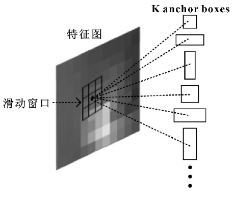
In order to generate accurate candidate regions, 512 feature maps are used as input of RPN (region proposal networks) and output as a series of rectangular target candidate regions. Firstly, the 3 * 3 convolution kernel is used as the sliding window to select the sliding window on the output feature map of convolution layer. As shown in Figure 1, there are several windows in the ferrography feature map, and each window generates K target candidate regions according to a certain proportion, which are called anchor boxes. Each pixel in the original image is the center of the sliding window. In this paper, according to the size of wear particles in ferrography image, each sliding window uses (1 ∶ 1, 1 ∶ 2, 2 ∶ 1) size and proportion to generate 9 anchor boxes. Each sliding window is mapped into 512 dimensional feature vectors of res net-34 network output, and then transmitted to two subnetworks: candidate box classification network and candidate box regression network. Therefore, each sliding window contains 18 outputs, that is, 512 dimensional vector is mapped to 18 dimensional vector. Sofmax classifier is used in the classification network

Where: J is the array; FYI is the ith value in the corresponding array J.
The loss function of classification network is as follows

Where: Pi is anchor boxes and predicted as Ferrography Wear Particles; p * I is prediction probability of target window. If IOU is more than 0.7, then p * I is 1, that is to say, it is judged that there are abrasive particles in the target frame; if IOU < 0.3, p * I is 0, which means that there are no abrasive particles in the target frame.
The output of the candidate frame regression network is 4 translation and scaling parameters, which makes the an chors boxes closer to the real abrasive area, that is, each sliding window contains 36 outputs. The translation and zoom scale of anchor boxes is as follows:

Where: WP and HP are the width and length of the predicted anchor boxes; Δ X and Δ y are the translation scale; Δ W and Δ h are the scaling scale; DX (P), Dy (P), DW (P), DH (P) are the four transformations to be learned. The objective function is set as follows:

Where: Φ (a) is the eigenvector composed of the characteristic graph of the convolution output; D * (a) is the four transformations in the formula; wt * is the parameter of linear regression learning.
In order to make the predicted value d * (a) closer to the real value t *, a loss function is designed

The objective of function optimization is as follows:

Where: n is the nth characteristic graph.
The gradient descent method is used to obtain w ∧ *, and the final wt * is learned to obtain the translation and scaling scale of the predicted anchor boxes, so that they are closer to the real abrasive region after transformation.

