
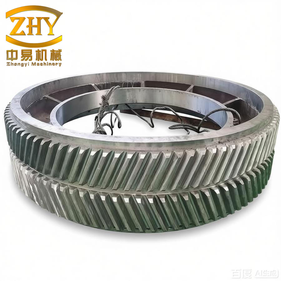
Herringbone gears are critical power transmission components widely used in aviation engines. In our research, we focused on the form grinding process of herringbone gears, which is the final and most essential manufacturing stage that determines the surface integrity and service performance of these components. The unique geometric structure of herringbone gears, characterized by two opposite-handed helical tooth flanks separated by a relief groove, brings significant difficulties to the grinding process. Low grinding efficiency, conservative process parameter selection, and poor coordination between design and manufacturing are longstanding problems in actual production. To address these issues, our research systematically investigated the grinding mechanism of herringbone gears, optimized the grinding process by proposing a novel borrow grinding method, and established a predictive model for grinding forces.
Our study revealed that the grinding wheel diameter is one of the most influential parameters affecting the grinding efficiency and surface quality of herringbone gears. A larger wheel diameter increases the contact length, improves heat dissipation, reduces wheel wear, and allows more dressing cycles. However, due to the compact structure of herringbone gears, the available space for the grinding wheel is severely limited by the width of the relief groove. Traditional methods for enlarging the wheel diameter usually require widening the relief groove, which directly contradicts the lightweight design requirements of aviation components. Therefore, we proposed a set of borrowing grinding methods that exploit the space of the opposite tooth groove, the opposite adjacent tooth groove, and the relief groove itself. These methods permit a considerable expansion of the grinding wheel diameter without increasing the relief groove width.
1. Introduction
In the manufacturing industry, the production capability of high-end components directly reflects the technical level and industrial competitiveness of a country. Herringbone gears, as key transmission parts in aero-engines, must meet stringent requirements in terms of dimensional accuracy, tooth surface quality, and mechanical performance under severe service conditions including high temperature, high speed, and heavy load. The manufacturing of herringbone gears involves multiple processes, among which grinding is indispensable to eliminate heat-treatment distortion, ensure final accuracy, and achieve the required surface finish.
Because of the high hardness and poor thermal conductivity of aerospace gear steels, grinding of herringbone gears is prone to excessive grinding zone temperature, severe wheel wear, and grinding burns. In practice, conservative grinding parameters are often adopted to protect the workpiece surface, which substantially reduces productivity. Moreover, the complex spatial relationships between the grinding wheel and the herringbone gear tooth surfaces make the grinding process difficult to model accurately.
In the field of gear design and manufacturing technology, extensive research has been carried out worldwide. Various scholars have established calculation models for the minimum relief groove width of herringbone gears as functions of the number of teeth, normal modulus, and helix angle. Parametric modeling methods have been developed to represent high-precision involute and tooth root transition curves of herringbone gears. Investigations on the exact cross-sectional profile of formed grinding wheels based on meshing principles have also been conducted. Additionally, tooth profile error prediction and compensation techniques have been proposed for helical gears in form grinding. However, these studies mainly focus on the geometry and dynamics of herringbone gears; the grinding process optimization and the collaborative design of herringbone gears considering manufacturing constraints remain insufficiently explored.
Regarding grinding force prediction, early research established empirical models that relate the grinding force to the material removal rate, wheel speed, and workpiece speed. Later, analytical models were developed by considering the undeformed chip thickness distribution based on the random arrangement of abrasive grains. Some researchers built grinding force models based on the contact mechanics of a single abrasive grain, considering elastic, plastic, and chip formation stages. More recent works have incorporated the wear state of the grains, the grain size distribution, and the dynamic effective grain density into the force models. Nevertheless, the application of these models to the specific case of herringbone gear form grinding has been limited. The tooth surface geometry of herringbone gears leads to a varying contact width along the tooth profile, and the grinding force model must reflect this variation.
In our research, the main objectives are summarized as follows: (1) to propose a quantitative borrow grinding method for herringbone gears; (2) to develop maximum grinding wheel diameter models for both relief groove borrowing and tooth groove borrowing under practical constraints; (3) to establish a grinding force prediction model based on the micro-interaction mechanisms of grain-workpiece at different material removal stages; and (4) to develop grinding process software that enables effective design-manufacturing collaboration for herringbone gears.
2. Borrow Grinding Technology of Herringbone Gears
2.1 Process requirements and the need for wheel diameter expansion
The structure of herringbone gears consists of two helical gear sections with opposite helical directions manufactured in one piece. A relief groove is machined between the two sections to provide tool clearance and avoid machining interference. In the grinding process, the grinding wheel must be aligned with the tooth slot of one helical section and fed in the direction of the gear axis. The width of the relief groove determines the maximum size of the grinding wheel that can pass through the groove without interfering with the adjacent tooth flanks.
From the viewpoint of production, a larger grinding wheel is always desirable because it provides a larger grinding contact area, higher linear speed at the same spindle speed, better cooling, and longer wheel life. The wheel diameter is thus a decisive factor for grinding efficiency and surface quality. However, in the case of herringbone gears used in aviation, the trend of miniaturization and weight reduction of transmission systems directly conflicts with the demand for larger grinding wheels. Reducing the relief groove width by merely 1 mm can save approximately 40 kg in weight for a single aero-engine, but it also reduces the accessible space for the grinding wheel.
In the conventional grinding mode, the grinding wheel can only pass through the relief groove directly without utilizing any extra space from the tooth slots. We observed through practical grinding experiments and numerical simulations that herringbone gears with appropriate helix angles and relief groove widths possess hidden spaces on the opposite side of the gear that are not exploited. This motivated us to propose a borrow grinding concept, in which the grinding wheel is offset or removed to borrow space from the opposite tooth groove or the opposite adjacent tooth groove, thus allowing a larger wheel diameter than the conventional limit.
2.2 Three forms of borrow grinding
The borrow grinding method for herringbone gears can be classified into three forms: (1) borrowing the opposite tooth groove; (2) borrowing the relief groove; and (3) borrowing the opposite adjacent tooth groove. The first form means that the grinding wheel, while grinding one tooth slot, partially enters the opposite tooth slot space of the same side. The second form corresponds to the conventional case where the wheel passes through the relief groove. The third form implies that the wheel additionally utilizes the space of the adjacent tooth-groove on the opposite side. The latter form is only applicable to herringbone gears without staggered teeth.
Our research quantified the possibility of borrow grinding using a dimensionless parameter, the borrowing coefficient K, derived from the geometric relationship on the pitch cylindrical surface.
2.3 Geometric modeling of key parameters
We modeled the key parameters of herringbone gears based on the geometric relationship on the pitch cylindrical surface. On this surface, a curved triangle formed by the intersection points of the tooth center lines and the gear axis can be established. The relationship among the relief groove width L, the helix angle β, the normal modulus mn, the tooth number Z, and the pitch radius R was derived. The arc length between the center points of two adjacent tooth slots on the pitch circle is related to the relief groove width and the helix angle.
Defining the borrowing coefficient K as the ratio of the arc length corresponding to the relief groove width to the circular pitch, we obtained:
$$ \frac{L}{\pi \cdot m_n} = \frac{K}{\sin \beta} $$
This equation indicates that for a given normal modulus and helix angle, the relief groove width is proportional to the borrowing coefficient. When K equals an integer, the grinding wheel can theoretically be aligned with a tooth slot on the opposite side. In practice, because the wheel thickness is slightly less than the tooth slot width, K can deviate from an integer within a certain range while still maintaining the borrowing condition.
To determine the feasible range of K, we introduced a profile deviation function H(K). By substituting the relationship of L into the geometric model, we derived:
$$ H = \frac{n_m \cdot K \cdot (Z – 1)}{\sin \beta \cdot \cos \beta} $$
Extensive numerical simulations and experiments showed that when K exceeds 3, the wheel profile and gear profile are sufficiently separated so that no interference occurs. Therefore, the meaningful range of the borrowing coefficient is (0, 3).
Furthermore, the feasible interval for tooth groove borrowing is bounded by Ka and Kb, which correspond to the intersections of the involute profile with the pitch circle. Considering the tooth side clearance Jt and the safety margin δ, we expressed these boundaries as:
$$ K_a = 0.75 – \frac{J_t}{S_p} + \delta $$
$$ K_b = 1.25 + \frac{J_t}{S_p} – \delta $$
where Sp is the circular pitch. Table 1 summarizes the physical meaning of different borrowing coefficient ranges.
| Range of K | Grinding wheel status | Borrowing evaluation |
|---|---|---|
| [0, 0.25) | Borrowing the opposite tooth groove | Rare; β is too small |
| [0.25, 0.75) | Interference with the opposite tooth profile | Not applicable for borrowing |
| [0.75, 1.25) | Borrowing the opposite adjacent tooth groove | Common; β ≈ (15°, 35°) |
| [1.25, 1.75) | Interference with the opposite adjacent profile | Not applicable for borrowing |
| [1.75, +∞) | No interference | Rare; β is too large |
The interval [0.75, 1.25) is the most significant range in practice. Within this interval, the grinding wheel can borrow the space of the opposite adjacent tooth groove without interfering with the gear tooth surfaces, which is the foundation of the proposed borrow grinding method.
2.4 Design and manufacturing collaboration based on borrow grinding
The introduction of the borrowing coefficient creates a bridge between design and manufacturing. From the design perspective, the relief groove width is a critical structural parameter for the weight of herringbone gears. From the manufacturing perspective, the maximum grinding wheel diameter is determined by the same parameter. Our research established a quantitative mapping between these two perspectives.
With a fixed borrowing coefficient of 1, which represents the theoretical optimum condition for borrowing, we constructed a mapping surface among L, β, and mn. This surface provides a visual tool for designers to determine the parameter combinations that allow grinding wheel borrowing. By appropriately adjusting the relief groove width, the helix angle, or the normal modulus, designers can realize the goal of lightweight design while ensuring that the herringbone gear can be ground using a larger wheel. Consequently, the proposed borrow grinding method plays a key role in the design-manufacturing collaboration of herringbone gears.
3. Maximum Grinding Wheel Diameter Modeling and Validation
3.1 Model of maximum wheel diameter in relief groove borrowing
To precisely determine the maximum allowable grinding wheel diameter for herringbone gears, we first developed the model for the conventional condition, i.e., relief groove borrowing. A grinding wheel with center O′ and radius Rw must pass through the relief groove of width L and then engage with the tooth slot on the opposite side of the gear. The geometric condition for avoiding interference is that the distance between the wheel center and the gear center must be greater than the sum of the wheel radius and the gear addendum radius.
Based on the law of cosines in the triangle formed by the gear center, the wheel center, and the contact point on the gear addendum circle, we derived the relationships among the geometric parameters:
$$ \begin{cases} ab = L \cdot \tan \beta \\ ac = \dfrac{L}{\cos \beta} \\ ao = \sqrt{R_u^2 + ab^2} \\ co = \sqrt{R_u^2 + L^2} \end{cases} $$
where Ru is the addendum circle radius. In triangle aoc, the angle at point a is obtained from:
$$ \cos \angle cao = \frac{ac^2 + ao^2 – co^2}{2 \cdot ac \cdot ao} $$
The distance cd between the contact point and the gear center is then given by:
$$ cd = \sqrt{ac^2 + ad^2 – 2 \cdot ac \cdot ad \cdot \cos \angle cao} $$
where ad = ao − Ru. In triangle dco′, the angle ∠dco′ is determined by considering the line segments gd and co′:
$$ \angle dco’ = \frac{\pi}{2} + \angle gcd $$
$$ \angle gcd = \arcsin\left( \frac{gd}{cd} \right) $$
$$ \begin{cases} gd = ad \cdot \cos \angle gda \\ \angle gda = \dfrac{2\pi}{Z} \end{cases} $$
By applying the law of cosines in triangle dco′, the maximum wheel diameter for relief groove borrowing is:
$$ D = \frac{2 \cdot cd \cdot h \cdot \cos(\angle dco’) + \sqrt{cd^2 + h^2 \cdot \cos^2(\angle dco’)}}{cd + h \cdot \cos(\angle dco’)} $$
where h represents the geometric distance parameter in the triangle model. This model provides a precise calculation of the maximum wheel diameter that can pass through the relief groove of a herringbone gear without interference.
3.2 Model of maximum wheel diameter in tooth groove borrowing
For tooth groove borrowing, the grinding wheel is allowed to utilize the space of the opposite adjacent tooth groove, resulting in a larger maximum wheel diameter DMax compared to the conventional relief groove borrowing. In this case, the geometric model becomes more complicated because the wheel center and the contact points do not lie on the same plane due to the helical twist of the gear teeth on the base cylindrical surface.
To account for the twisting deformation, we introduced the curved triangle d″ne′ and computed the additional depth df′ that the wheel can penetrate into the tooth space:
$$ \begin{cases} ee’ = w \cdot \tan \beta \cdot \left( \frac{R_u}{R} \cdot \frac{2\pi}{Z} – 1 \right) \\ en = \dfrac{2 \cdot \sin \beta \cdot R_u}{w} \\ e’n = en + ee’ + en \cdot ee’ \end{cases} $$
In triangle f′de′, the total penetration depth df′ is:
$$ df’ = \frac{ne’ \cdot e’d \cdot \sin(\angle ne’e)}{\cos(\lambda_{ne’e} – \beta)} $$
The intermediate variables are:
$$ \begin{cases} \angle ne’e = \arcsin\left( \dfrac{w}{e’n} \right) \\ e’d = e’e + ed \end{cases} $$
Because of the helical twist, the point f on the tooth flank is radially displaced to point f′. The displacement is:
$$ \Delta f = \sqrt{(df’ \cdot \sin \beta)^2 + R_u^2} – R_u $$
The angle between the segments cd and cf is:
$$ \angle fcf’ = \arctan\left( \frac{-\Delta f}{df’ – cd} \right) $$
After computing the geometric parameters, the maximum wheel diameter for tooth groove borrowing is derived as:
$$ D_{Max} = \frac{2 \cdot f’c \cdot h \cdot \cos(\angle f’co’) + \sqrt{f’c^2 + h^2 \cdot \cos^2(\angle f’co’)}}{f’c + h \cdot \cos(\angle f’co’)} $$
where:
$$ \begin{cases} \angle f’co’ = \angle fcf’ + \angle fco’ \\ f’c = \dfrac{df’ + cd}{\cos \angle fcf’} \end{cases} $$
The model was further verified through contact simulations and machining trials, as described in the following sections.
3.3 Model modification and compensation
3.3.1 Compensation for wheel thickness and tooth side clearance
In practical applications, the actual thickness of the grinding wheel is generally smaller than the tooth slot width. Additionally, the tooth side clearance and the profile modification of the tooth flanks affect the available borrowing space. To avoid complex analytical expressions for the contact interference cases, we constructed correction coefficient functions U and V based on the simulation results:
$$ U = \cos(2\pi \cdot K) \cdot |K – 1| $$
$$ V = \frac{L}{\sin \beta} \cdot |K – 1| $$
The corrected segment f′c is:
$$ FC = \frac{U \cdot df’ + V \cdot cd}{\cos(\angle fcf’)} $$
The final expression for the maximum wheel diameter in tooth groove borrowing is then:
$$ D_{Max} = \frac{2 \cdot FC \cdot h \cdot \cos(\angle f’co’) + \sqrt{FC^2 + h^2 \cdot \cos^2(\angle f’co’)}}{FC + h \cdot \cos(\angle f’co’)} $$
3.3.2 Over-center grinding compensation
When grinding the tooth surface of herringbone gears, the grinding wheel must not only pass through the relief groove but also perform an over-center movement to ensure that the entire tooth flank is ground. This requires an additional space DE in the axial direction. We calculated the required lifting space as:
$$ \begin{cases} D_E = C_{cn} \cdot \sin \beta \\ L_E = C_{cn} \cdot \sin \beta \cdot \cos \beta \end{cases} $$
where Ccn is the half chordal thickness of the addendum circle:
$$ C_{cn} = R_u \cdot \sin\left( \frac{\pi}{2} – \frac{S_u}{Z \cdot R_u} \right) $$
This compensation is essential for practical implementation of the borrow grinding method. The compensated diameter models are:
$$ \begin{cases} D = \dfrac{2 \cdot cd \cdot (D_E + h) \cdot \cos(\angle dco’) + \sqrt{cd^2 + (D_E + h)^2 \cdot \cos^2(\angle dco’)}}{cd + (D_E + h) \cdot \cos(\angle dco’)} \\ D_{Max} = \dfrac{2 \cdot FC \cdot (D_E + h) \cdot \cos(\angle f’co’) + \sqrt{FC^2 + (D_E + h)^2 \cdot \cos^2(\angle f’co’)}}{FC + (D_E + h) \cdot \cos(\angle f’co’)} \end{cases} $$
3.4 Simulation validation
We performed solid contact simulations using commercial CAD software for twelve typical herringbone gear models to validate the developed models. The structural parameters of these gears are listed in Table 2.
| Gear | mn (mm) | β (°) | α (°) | Z | W (mm) | L (mm) | φu (mm) | φd (mm) |
|---|---|---|---|---|---|---|---|---|
| 1 | 3.81 | 30 | 22.5 | 23 | 41 | 19 | 110.41 | 118.50 |
| 2 | 3.81 | 30 | 22.5 | 88 | 41 | 19 | 517.33 | 525.30 |
| 3 | 2.93 | 30 | 22.5 | 20 | 42 | 19 | 81.21 | 78.15 |
| 4 | 2.93 | 30 | 22.5 | 116 | 42 | 19 | 302.18 | 218.50 |
| 5 | 3.12 | 30 | 22.5 | 30 | 28 | 19 | 100.16 | 90.81 |
| 6 | 3.12 | 30 | 22.5 | 105 | 28 | 19 | 360.12 | 308.20 |
| 7 | 3.17 | 30 | 22.5 | 31 | 51 | 19 | 150.10 | 111.40 |
| 8 | 3.17 | 30 | 22.5 | 90 | 51 | 19 | 636.22 | 617.20 |
| 9 | 6.00 | 30 | 22.5 | 24 | 38 | 19 | 155.10 | 117.80 |
| 10 | 5.00 | 30 | 22.5 | 21 | 38 | 19 | 141.78 | 113.10 |
| 11 | 3.11 | 30 | 22.5 | 26 | 13.6 | 14 | 67.25 | 62.98 |
| 12 | 2.11 | 30 | 22.5 | 38 | 13.6 | 14 | 88.55 | 83.33 |
The intermediate variable DE was verified by comparing the model calculation with the simulation result, as shown in Table 3. The average relative error was 4.45%, which satisfies the modeling requirements.
| Gear | DE (mm) | DE′ (mm) | Error (%) |
|---|---|---|---|
| 1 | 3.183 | 3.281 | 2.987 |
| 2 | 2.771 | 3.000 | 7.633 |
| 3 | 2.181 | 2.168 | 0.600 |
| 4 | 1.711 | 1.911 | 10.466 |
| 5 | 1.987 | 2.073 | 4.149 |
| 6 | 1.862 | 1.954 | 4.708 |
| 7 | 3.088 | 3.221 | 4.129 |
| 8 | 2.872 | 3.012 | 4.648 |
| 9 | 3.005 | 3.040 | 1.151 |
| 10 | 2.911 | 3.031 | 3.959 |
| 11 | 1.137 | 1.174 | 3.152 |
| 12 | 1.077 | 1.143 | 5.774 |
Table 4 compares the calculated maximum wheel diameters D and DMax with the simulation results for all twelve gears.
| Gear | K | Judgment | D (mm) | D′ (mm) | Error (%) | DMax (mm) | D′Max (mm) | Error (%) |
|---|---|---|---|---|---|---|---|---|
| 1 | 0.721 | Yes | 48.745 | 49.195 | 0.915 | 64.334 | 68.00 | 5.391 |
| 2 | 0.721 | Yes | 48.938 | 48.186 | 1.573 | 59.037 | 63.00 | 6.290 |
| 3 | 1.166 | No | 80.705 | 86.609 | 6.817 | — | — | — |
| 4 | 1.166 | No | 75.974 | 75.051 | 0.132 | — | — | — |
| 5 | 1.158 | Yes | 90.617 | 93.961 | 3.559 | 118.422 | 128.159 | 7.598 |
| 6 | 1.158 | Yes | 82.469 | 82.514 | 0.055 | 100.243 | 102.660 | 2.354 |
| 7 | 0.749 | Yes | 53.629 | 53.979 | 0.648 | 53.691 | 52.00 | 3.252 |
| 8 | 0.749 | Yes | 52.872 | 52.462 | 0.782 | 52.764 | 55.00 | 4.065 |
| 9 | 0.796 | Yes | 56.588 | 57.341 | 1.313 | 67.520 | 67.00 | 0.776 |
| 10 | 0.796 | Yes | 57.320 | 57.728 | 0.707 | 68.150 | 68.00 | 0.221 |
| 11 | 1.530 | No | 103.596 | 111.467 | 7.061 | — | — | — |
| 12 | 1.530 | No | 96.946 | 100.921 | 3.939 | — | — | — |
The relative errors of D and DMax are all below 10%, with average errors of 3.43% and 3.74%, respectively. The inward convergence error caused by the assumptions and simplifications is about 3.59%, which is acceptable for both theoretical analysis and practical application.
3.5 Experimental validation
We conducted trial grinding and contact experiments on a Klingelnberg CNC gear grinding machine. To protect the finished tooth surfaces from scratches, we used bakelite model grinding wheels. Two new herringbone gears, Gear 13 and Gear 14, were employed for the contact verification. The parameters and the calculated maximum diameters are given in Table 5.
| Gear | mn (mm) | β (°) | α (°) | Z | L (mm) | φu (mm) | φd (mm) | K | D (mm) | DMax (mm) |
|---|---|---|---|---|---|---|---|---|---|---|
| 13 | 1.6 | 28 | 22.5 | 29 | 17 | 56.34 | 48.442 | 1.64 | 149.8084 | — |
| 14 | 1.5 | 25 | 22.5 | 55 | 13 | 99.91 | 101.128 | 1.19 | 48.2082 | 54.7443 |
For Gear 13, the model wheel diameter was dressed to 150 mm. The difference between the theoretical diameter D = 149.8084 mm and the practical value was only 0.13%. For Gear 14, the model wheel diameter was reduced to 55 mm. The calculated DMax = 54.7443 mm showed an error of only 0.46% compared to the practical value. These results strongly validate the accuracy of the developed models.
In actual production, twelve typical types of herringbone gears have been successfully ground using the borrow grinding process. Table 6 compares the production grinding wheel diameter DA with the calculated D and DMax values.
| Gear | D (mm) | DMax (mm) | DA (mm) |
|---|---|---|---|
| 1 | 48.745 | 64.334 | 63 |
| 2 | 48.938 | 59.037 | 54 |
| 3 | 80.705 | — | 66 |
| 4 | 75.974 | — | 64 |
| 5 | 90.617 | 118.422 | 67 |
| 6 | 82.469 | 100.243 | 68 |
| 7 | 53.629 | 53.691 | 55 |
| 8 | 52.872 | 52.760 | 53 |
| 9 | 56.588 | 67.520 | 65 |
| 10 | 57.320 | 68.150 | 65 |
| 11 | 103.596 | — | 64 |
| 12 | 96.946 | — | 65 |
3.6 Discussion of the validation results
The validation results show that the borrow grinding method can significantly increase the maximum grinding wheel diameter for herringbone gears, as summarized in Table 7. The improvement depends strongly on the borrowing coefficient K.
| Gear | K | (Ka, Kb) | D (mm) | DMax (mm) | Improvement (%) |
|---|---|---|---|---|---|
| 1 | 0.821 | (0.746, 1.254) | 48.745 | 64.334 | 31.981 |
| 2 | 0.821 | (0.746, 1.254) | 48.938 | 59.037 | 20.636 |
| 5 | 1.158 | (0.746, 1.255) | 90.617 | 118.422 | 30.684 |
| 6 | 1.158 | (0.745, 1.255) | 82.469 | 100.243 | 21.552 |
| 7 | 0.749 | (0.747, 1.253) | 53.629 | 53.691 | 0.116 |
| 8 | 0.749 | (0.747, 1.253) | 52.872 | 52.764 | -0.204 |
| 9 | 0.796 | (0.747, 1.253) | 56.588 | 67.520 | 19.319 |
| 10 | 0.796 | (0.747, 1.253) | 57.320 | 68.150 | 18.894 |
For Gears 5 and 6, the wheel diameter without borrowing is already relatively large, and the improvement from tooth groove borrowing is significant. However, if the actual production wheel diameter is limited by the machine tool specifications, the same model can be used conversely to reduce the relief groove width while maintaining the desired wheel diameter. Table 8 shows that the relief groove width of Gears 5 and 6 can be reduced by 22.48% and 18.55%, respectively, when the wheel diameter is limited to 78 mm.
| Gear | φu (mm) | L (mm) | DMax (mm) | DA (mm) | L′ (mm) | Reduction (%) |
|---|---|---|---|---|---|---|
| 5 | 100.16 | 19 | 118.422 | 78 | 15.504 | 22.48 |
| 6 | 360.12 | 19 | 100.243 | 78 | 16.290 | 18.55 |
It should also be noted that not all borrowable herringbone gears are suitable for the borrowing operation. For Gears 7 and 8, the borrowing coefficient 0.749 is very close to the boundary 0.747, and the tooth groove borrowing yields almost no benefit or even a negative effect due to the wheel thickness interference. In such cases, the safety margin δ should be set to at least 0.002 to prevent the use of tooth groove borrowing.
4. Grinding Force Prediction Modeling of Herringbone Gears
4.1 Fundamental modeling of the single-grain grinding process
Grinding force is not only the most important physical quantity characterizing the grinding process but also the basis for analyzing the grinding mechanism of herringbone gears. The grinding force is composed of three stages: sliding, ploughing, and chip formation. In the sliding stage, the abrasive grain rubs against the workpiece surface, causing elastic deformation. In the ploughing stage, the workpiece material undergoes plastic deformation and is pushed to the sides of the groove. In the chip formation stage, the material is actually removed in the form of chips. Our grinding force model separately calculates the contribution of each stage.
The total normal and tangential grinding forces for herringbone gears are expressed as:
$$ F_t = F_{ts} + F_{tp} + F_{tc} $$
$$ F_n = F_{ns} + F_{np} + F_{nc} $$
4.2 Abrasive grain morphology and effective contact angle
The surface of the grinding wheel contains randomly distributed abrasive grains of different shapes and sizes. In our model, the grains are simplified as regular cones. The spatial position relationship between adjacent grains in the grinding direction can be represented as a double-grain group. Due to the staggered arrangement of the grains, the front grain may shield part of the rear grain from contacting the workpiece. This shielding effect significantly affects the effective contact angle of the rear grain. According to the relative positions of the two grains, we divided the effective contact angle into four intervals, as listed in Table 9.
| Case | Effective contact angle range | Physical condition |
|---|---|---|
| 1 | [−π/2, −π/4] | Severe shielding by the front grain |
| 2 | [−π/2, 0] | Moderate shielding |
| 3 | [−π/2, π/4] | Slight shielding |
| 4 | [−π/2, π/2] | Almost no shielding |
The integration of the force components over these intervals allows us to account for the randomness of grain distribution without requiring an explicit model of each individual grain orientation.
4.3 Sliding stage grinding force model
In the sliding stage, the workpiece material undergoes elastic deformation. The contact stress is calculated based on the Hertz contact theory. The dynamic effective grain number in the sliding stage is:
$$ N_{ts} = \xi_s \cdot N_d \cdot \sqrt{a_p \cdot d_s} \cdot b_c $$
The grinding contact width along the herringbone gear tooth profile varies with the pressure angle α:
$$ b_c = \frac{2 \cdot m_n \cdot (h^* + c^*)}{(\cos \alpha)^{-1}} $$
The normal sliding force is then:
$$ F_{ns} = \xi_s \cdot N_d \cdot \sqrt{a_p \cdot d_s} \cdot \frac{E_2 \cdot \cos \theta \cdot m_n \cdot (2h^* + c^*)}{(1 – V^2) \cdot 2 \sin \theta \cdot (\cos \alpha)^{-1}} $$
The friction coefficient in the sliding stage is expressed as:
$$ \mu_s = \lambda_1 + \frac{\lambda_2 \cdot A_1}{F_{ns}} $$
where A1 is the wear flat area. The tangential sliding force is:
$$ F_{ts} = \mu_s \cdot F_{ns} \cdot N_{ts} $$
4.4 Ploughing stage grinding force model
In the ploughing stage, plastic deformation dominates. By integrating the differential force components on a single grain over the four effective contact angle intervals, we obtained four sets of tangential and normal ploughing force equations. The differential force components on a single grain are:
$$ \mathrm{d}F_{tp} = \frac{1}{2} F_p l_c^2 \sin \theta \cos \theta \cos \varphi \, \mathrm{d}\varphi $$
$$ \mathrm{d}F_{np} = \frac{1}{2} F_p l_c^2 \sin^2 \theta \cos \theta \cos \varphi \, \mathrm{d}\varphi $$
where Fp is the effective ploughing stress. Integrating over the four intervals gives:
$$ F_{tp1} = F_p l_c^2 \sin \theta \cos \theta \left( \frac{\pi}{16} – \frac{1}{8} \right) $$
$$ F_{tp2} = F_p l_c^2 \sin \theta \cos \theta \cdot \frac{\pi}{8} $$
$$ F_{tp3} = F_p l_c^2 \sin \theta \cos \theta \left( \frac{3\pi}{16} + \frac{1}{8} \right) $$
$$ F_{tp4} = F_p l_c^2 \sin \theta \cos \theta \cdot \frac{\pi}{4} $$
and for the normal component:
$$ F_{np1} = F_p l_c^2 \sin^2 \theta \cos \theta \left( \frac{1}{4} – \frac{1}{2\pi} \right) $$
$$ F_{np2} = \frac{1}{2} F_p l_c^2 \sin^2 \theta \cos \theta $$
$$ F_{np3} = F_p l_c^2 \sin^2 \theta \cos \theta \left( \frac{1}{4} + \frac{1}{2\pi} \right) $$
$$ F_{np4} = F_p l_c^2 \sin^2 \theta \cos \theta $$
The dynamic effective grain number in the ploughing stage is:
$$ N_{tp} = \xi_p \cdot N_d \cdot \sqrt{a_p \cdot d_s} \cdot b_c $$
Therefore, the total ploughing forces corresponding to the four contact cases are obtained by multiplying Ntp with the corresponding single-grain force components.
4.5 Chip formation stage grinding force model
In the chip formation stage, material is removed by shear deformation. The grinding specific energy u is defined as:
$$ u = \frac{F_{tc} \cdot v_s}{b_c \cdot v_w \cdot a_p} $$
Based on the shear deformation theory, the shear strain and shear strain rate are:
$$ \gamma = \frac{\cos \theta}{\sin \varphi \cdot \cos(\varphi – \theta)} $$
$$ \dot{\gamma} = \frac{v_s \cdot \cos \theta}{2 \cdot R \cdot \sin \varphi \cdot \cos(\varphi – \theta)} $$
The shear stress is related to the strain rate through:
$$ \mu = \lambda_5 \cdot \ln \dot{\gamma} $$
The tangential grinding force in the chip formation stage is:
$$ F_{tc} = N_{tc} \cdot \frac{\lambda_5 \lambda_6 \ln(\dot{\gamma}) \cdot a_p \cdot v_w \cdot b_c}{v_s} + \mu_c \cdot H \cdot S $$
where μc is the friction coefficient in the chip formation stage, H is the workpiece hardness, and S is the contact area. The normal grinding force is:
$$ F_{nc} = N_{tc} \cdot \frac{\lambda_5 \lambda_6 \lambda_7 \ln(\dot{\gamma}) \cdot a_p \cdot v_w \cdot b_c}{v_s} + (\alpha_0 + \beta_0) \cdot P \cdot H \cdot S $$
All coefficients λ and α,β are determined by the physical and mechanical properties of the contact materials and are calibrated through experiments.
5. Form Grinding Experiments and Grinding Process Software
5.1 Experimental setup and parameters
To validate the grinding force prediction model, we conducted form grinding experiments on a Klingelnberg CNC gear grinding machine. The grinding wheel was a quartz wheel with parameters listed in Table 10. The workpiece was made of 9130 steel, and its structural parameters are given in Table 11.
| Material | Diameter (mm) | Width (mm) | Bore (mm) | Grit size |
|---|---|---|---|---|
| Quartz | 60 | 20 | 12 | 60 |
| Parameter | Value |
|---|---|
| Normal modulus (mm) | 1.7 |
| Helix angle (°) | 27 |
| Pressure angle (°) | 22.5 |
| Number of teeth | 67 |
| Face width (mm) | 15 |
| Relief groove width (mm) | 14 |
| Addendum circle diameter (mm) | 131.312 |
| Root circle diameter (mm) | 120.628 |
During the experiments, a Kistler 9257B dynamometer was used to measure the grinding force components. The grinding fluid was supplied continuously. The experimental process parameters are listed in Table 12.
| Feed rate (mm/min) | Grinding depth (mm) | Wheel speed (m/s) | Grinding allowance (mm) |
|---|---|---|---|
| 1000–3000 | 0.001–0.05 | 20–40 | 0.19 |
5.2 Comparison of predicted and measured grinding forces
Twenty groups of grinding experiments were conducted at randomly selected process parameters. The measured and predicted normal and tangential grinding forces are listed in Table 13.
| No. | vs (m/s) | vw (mm/min) | ap (mm) | Fn exp. (N) | Fn pred. (N) | Ft exp. (N) | Ft pred. (N) |
|---|---|---|---|---|---|---|---|
| 1 | 25 | 1200 | 0.008 | 15.4 | 14.5 | 25.3 | 27.3 |
| 2 | 28 | 1500 | 0.012 | 12.5 | 13.6 | 28.6 | 31.5 |
| 3 | 32 | 1800 | 0.015 | 25.6 | 27.7 | 32.8 | 36.8 |
| 4 | 35 | 2000 | 0.020 | 15.8 | 13.7 | 35.4 | 38.6 |
| 5 | 27 | 2200 | 0.025 | 10.6 | 9.57 | 38.2 | 43.5 |
| 6 | 31 | 2500 | 0.030 | 13.7 | 15.1 | 41.6 | 45.2 |
| 7 | 34 | 2800 | 0.035 | 22.3 | 24.1 | 44.9 | 49.6 |
| 8 | 29 | 3000 | 0.040 | 17.1 | 18.2 | 47.4 | 53.2 |
| 9 | 26 | 1300 | 0.010 | 14.9 | 17.1 | 26.5 | 29.2 |
| 10 | 33 | 1600 | 0.018 | 25.1 | 27.9 | 33.8 | 38.6 |
| 11 | 30 | 1900 | 0.022 | 7.7 | 8.9 | 37.7 | 40.6 |
| 12 | 36 | 2100 | 0.028 | 9.3 | 10.1 | 40.5 | 45.2 |
| 13 | 28 | 2400 | 0.032 | 28.1 | 30.2 | 43.6 | 47.3 |
| 14 | 34 | 2600 | 0.038 | 22.1 | 24.2 | 46.2 | 52.1 |
| 15 | 32 | 2900 | 0.042 | 13.6 | 15.4 | 48.3 | 53.2 |
| 16 | 27 | 1400 | 0.014 | 19.1 | 21.6 | 29.6 | 33.6 |
| 17 | 35 | 1700 | 0.016 | 9.6 | 11.1 | 34.8 | 37.6 |
| 18 | 31 | 2300 | 0.024 | 27.1 | 29.8 | 39.4 | 44.1 |
| 19 | 29 | 2700 | 0.034 | 25.8 | 27.1 | 44.8 | 49.1 |
| 20 | 33 | 3000 | 0.045 | 14.8 | 16.7 | 49.6 | 55.7 |
The comparison shows that the average error of the tangential grinding force is 10.34%, and that of the normal grinding force is 10.73%. The errors are within an acceptable range, which proves the effectiveness and reliability of the proposed grinding force model of herringbone gears. The influence of the grinding depth is the most significant among all parameters, followed by the feed rate and wheel speed.
We also measured the surface roughness of the ground tooth flanks. The average Ra obtained with our model-based parameters was approximately 0.3 μm, which is lower than the values of 0.46 μm, 0.48 μm, and 0.5 μm found with other grinding force models under the same machining conditions. This demonstrates that the proposed grinding force model contributes to improved surface quality of herringbone gears.
5.3 Development of grinding process software
To solidify the research results and facilitate practical application, we developed grinding process software using Python. The software consists of two modules: the borrow grinding discrimination module and the collaborative design processing module. The former judges whether a herringbone gear can be processed by the borrow grinding method and calculates the maximum wheel diameter. The latter calculates the optimal relief groove width for a given wheel diameter through a genetic algorithm, thereby supporting lightweight design of herringbone gears.
The software has been applied in actual production. Table 14 shows a representative case of the borrow discrimination module.
| Type | mn (mm) | β (°) | α (°) | Z | L (mm) | W (mm) | φu (mm) | φd (mm) |
|---|---|---|---|---|---|---|---|---|
| 1 | 1.65 | 30 | 22.5 | 20 | 17 | 15 | 65.402 | 57.472 |
| 2 | 1.65 | 30 | 22.5 | 58 | 17 | 15 | 131.92 | 111.72 |
| 3 | 3.414 | 30 | 22.5 | 96 | 17 | 30 | 310.68 | 288.55 |
| Type | Borrowing situation | D (mm) | DA (mm) | Error (%) |
|---|---|---|---|---|
| 1 | Not applicable | 149.31 | 150 | 0.46 |
| 2 | Not applicable | 115.38 | 116 | 0.53 |
| 3 | Applicable | 75.35 | 75.18 | 0.24 |
In the collaborative design module, a typical case involves a pinion with mn = 5.4 mm, β = 10.25°, α = 25°, Z = 19, and face width W = 90 mm. For a required wheel diameter of 124 mm, the minimum relief groove width was calculated to be 36.95 mm. Considering a safety margin, the design relief groove width was set to 39 mm, resulting in a maximum actual wheel diameter of 130.83 mm. For a large gear with Z = 180, the minimum wheel diameter was set to 300 mm, with a corresponding minimum relief groove width of 58.74 mm and a design value of 61 mm, enabling a maximum wheel diameter of 310.67 mm.
The software greatly shortens the time for determining the optimum grinding wheel size. In traditional practice, repeated machine trials and manual inspections took about 4 to 5 hours to determine the wheel size for a new herringbone gear type. With the grinding process software, the calculation, wheel dressing, and a single trial cut can be completed in about 0.5 hours. This substantial improvement demonstrates the practical value of our research for the production of herringbone gears.
Conclusion
In this research, we investigated the form grinding mechanism and process optimization of herringbone gears. The main conclusions are as follows:
(1) We proposed a borrow grinding method that allows the grinding wheel to utilize the opposite tooth groove, the opposite adjacent tooth groove, and the relief groove space. The borrowing coefficient K was defined as a dimensionless indicator to quantify the feasibility of gear-groove space borrowing. The interval [0.75, 1.25) was identified as the most significant range for practical applications. This method improves the grinding efficiency of herringbone gears without any change in the relief groove width.
(2) We established the maximum wheel diameter models for both the relief groove borrowing condition and the tooth groove borrowing condition. The models were corrected by considering the wheel thickness, the tooth side clearance, and the over-center grinding compensation. The average relative errors of the models were 3.43% and 3.74%, respectively, which were verified through contact simulation and actual machining experiments. The inward convergence error introduced by the modeling assumptions was approximately 3.59%.
(3) We developed a grinding force prediction model for herringbone gears based on the variable stages of grain-workpiece micro-interactions. The effective contact angle of the double-grain group was divided into four intervals, covering different shielding conditions of the grains. The sliding, ploughing, and chip formation stages were modeled separately. The experimental results showed that the average errors of the tangential and normal grinding forces were 10.34% and 10.73%, respectively, meeting the modeling accuracy requirements. The measured surface roughness of the ground herringbone gear tooth flanks also confirmed the practical applicability of the model.
(4) We developed grinding process software with a borrow grinding discrimination module and a collaborative design processing module. The software has been successfully applied in actual production, improving the grinding efficiency of herringbone gears and promoting the integration of design and manufacturing processes.
Future research may extend the current framework by incorporating grinding temperature analysis and wheel wear evolution into the grinding force model, which would further improve the theoretical completeness and engineering applicability of the research results on herringbone gears.