
I study the meshing behavior and vibration reduction of a helical gear pair used in the first reduction stage of a six-speed automatic transmission. My work connects an analytical helical gear mesh stiffness model, a robust tooth surface modification strategy, a coupled gear–bearing–rotor dynamic model, and order-tracking noise experiments. The central aim is to reduce the transmission whine caused by the first reduction helical gear pair without sacrificing load capacity or contact uniformity.
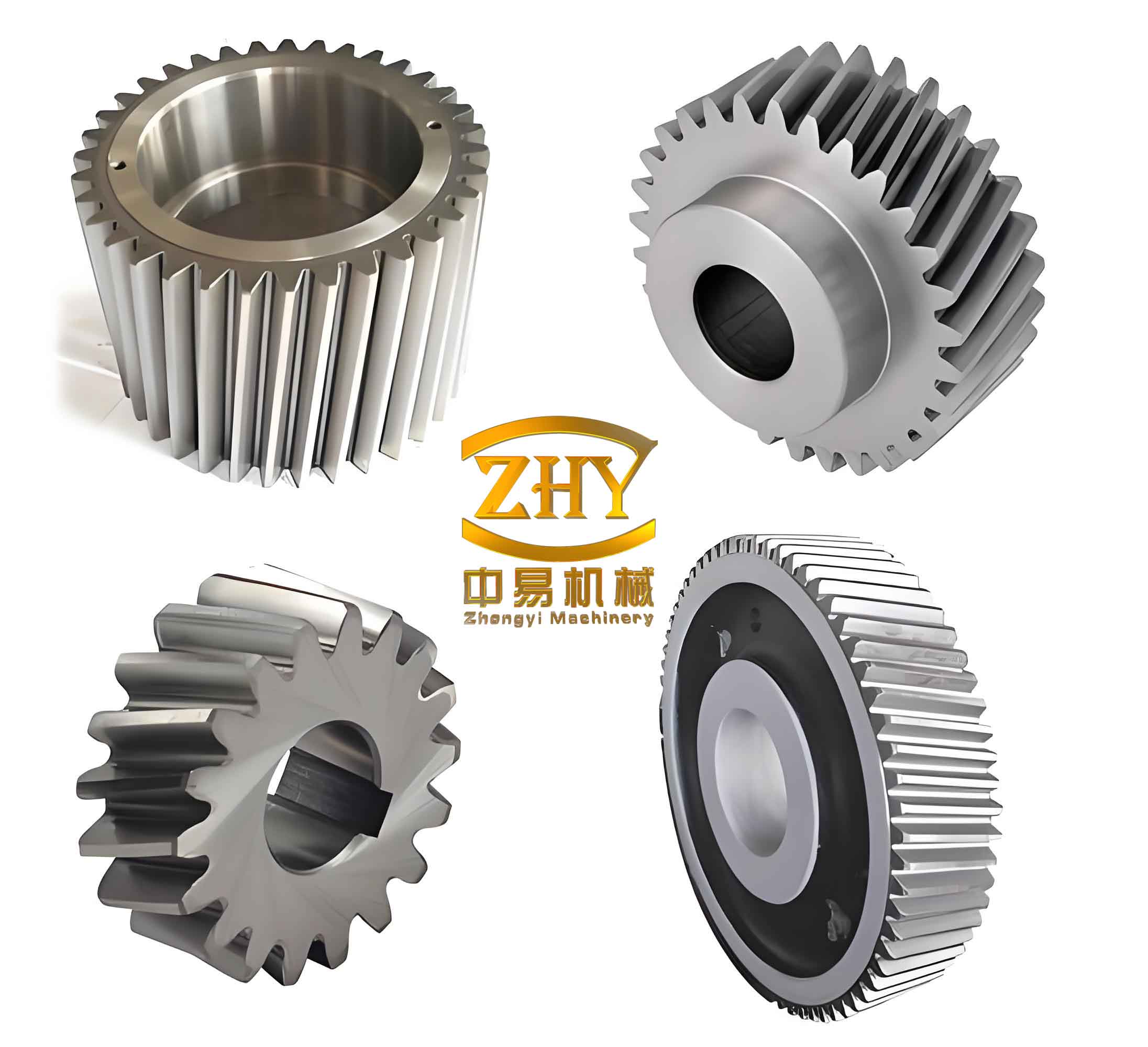
I treat the helical gear pair as the main internal excitation source of the transmission. In my model, the helical gear mesh stiffness and transmission error are not treated as constants. They vary with the contact line evolution, the torque level, the tooth profile modification, and the lead modification. I therefore build a chain of models in which the helical gear contact state drives the transmission error, the transmission error drives the dynamic response, and the dynamic response is finally checked against measured order noise.
1. Research Background and Motivation
Vehicle comfort has become a major evaluation index for modern automobiles. Noise, vibration, and harshness performance directly affects the perceived quality of a transmission. Among transmission components, the first reduction helical gear pair often dominates the whine noise because it carries high torque and operates over a wide speed range. I define the order of a rotating component as
$$O=\frac{f}{f_{0}}$$
where \(f\) is the frequency of interest and \(f_{0}\) is the reference shaft rotation frequency. For a helical gear pair, the mesh order is determined by the gear tooth number. If the driving helical gear has \(z_1\) teeth, the mesh order is \(z_1\). The first few mesh harmonics, such as \(2z_1\), \(3z_1\), and \(4z_1\), can also be visible in the measured noise spectrum. My experimental observations confirm that reducing the transmission error peak-to-peak value and the maximum tooth contact load of the helical gear pair is an effective way to reduce these order components.
I summarize the main NVH-related targets of my study in Table 1.
| Target | Physical meaning | Desired trend |
|---|---|---|
| Transmission error peak-to-peak value | Difference between maximum and minimum loaded transmission error over one mesh cycle | Minimize |
| Maximum tooth contact load | Highest distributed load among all helical gear contact points | Minimize and equalize |
| Mesh order noise | Noise at the helical gear mesh order and its harmonics | Minimize |
| Robustness over torque | Stability of the objective functions under variable torque | Maximize |
| Contact uniformity | Even load sharing along the helical gear tooth surface | Maximize |
2. Analytical Mesh Stiffness Model for Helical Gear Pairs
I begin with the stiffness of a single tooth slice. Using the slice method, I divide the helical gear along the face width into many thin slices. Each slice is treated as a spur gear slice with a small width. The total helical gear mesh stiffness is then obtained by accumulating the contributions of all active contact points along the contact line. This approach allows me to include the influence of the helical angle, the contact line length, and the overlap ratio without relying only on empirical formulas.
For one tooth slice, I consider five energy components: bending energy, shear energy, radial compression energy, Hertzian contact energy, and gear body energy. I write the total potential energy as
$$U_{\text{total}}=U_{b}+U_{s}+U_{a}+U_{h}+U_{f}$$
The corresponding stiffness components satisfy
$$\frac{1}{k_{\text{total}}}=\frac{1}{k_{b}}+\frac{1}{k_{s}}+\frac{1}{k_{a}}+\frac{1}{k_{h}}+\frac{1}{k_{f}}$$
I define the bending stiffness \(k_b\), shear stiffness \(k_s\), radial compression stiffness \(k_a\), Hertzian contact stiffness \(k_h\), and gear body stiffness \(k_f\) as follows:
$$k_{b}=\left[\int_{0}^{d}\frac{(d-x)\cos\alpha_{1}-h\sin\alpha_{1}}{EI_{x}}\,dx\right]^{-1}$$
$$k_{s}=\left[\int_{0}^{d}\frac{6\cos^{2}\alpha_{1}}{5GA_{x}}\,dx\right]^{-1}$$
$$k_{a}=\left[\int_{0}^{d}\frac{\sin^{2}\alpha_{1}}{EA_{x}}\,dx\right]^{-1}$$
$$k_{h}=\frac{\pi E b_{0}}{4(1-\nu^{2})}$$
$$k_{f}=\frac{E b_{0}}{L^{*}\left(\frac{\mu_{f}}{S_{f}}\right)^{2}+M^{*}\frac{\mu_{f}}{S_{f}}+P^{*}\tan\alpha_{1}+Q^{*}}$$
In these expressions, \(E\) is the elastic modulus, \(G\) is the shear modulus, \(b_0\) is the effective face width, \(\nu\) is Poisson’s ratio, \(I_x\) is the area moment of inertia, \(A_x\) is the cross-sectional area, and \(L^{*},M^{*},P^{*},Q^{*}\) are gear body coefficients. I use the standard involute and trochoid geometry to convert the tooth profile angle into the local coordinate along the tooth.
I list the basic helical gear parameters in Table 2.
| Parameter | Driving helical gear | Driven helical gear |
|---|---|---|
| Number of teeth | 53 | 63 |
| Normal module \(m_n\) (mm) | 2.0 | 2.0 |
| Normal pressure angle \(\alpha_0\) (deg) | 14.5 | 14.5 |
| Helical angle \(\beta_b\) (deg) | 27 | 27 |
| Total contact ratio \(\varepsilon_{\gamma}\) | 3.0 | 3.0 |
| Face width (mm) | 20 | 20 |
The helical gear contact line changes length during the meshing cycle. I divide the meshing behavior into three cases based on the transverse contact ratio \(\varepsilon_{\alpha}\) and the axial contact ratio \(\varepsilon_{\beta}\). The contact line length \(l(t)\) can be expressed in a piecewise form. For the case \(\varepsilon_{\alpha}>\varepsilon_{\beta}\), I use
$$l(t)=
\begin{cases}
l_{\max}\dfrac{t}{t_1}, & 0\le t<t_1\\[4pt] &="" <p="" \end{cases}$$="" l_{\max},="" l_{\max}\dfrac{t_m-t}{t_1},="" t<t_m="" tFor the case \(\varepsilon_{\alpha}=\varepsilon_{\beta}\), the contact line reaches its maximum at the mid-cycle. For the case \(\varepsilon_{\alpha}<\varepsilon_{\beta}\), the contact line has a different piecewise shape. In my model, the total contact ratio is 3.0, and the transverse contact ratio is larger than the axial contact ratio, so I use the first case for the first reduction helical gear pair.
I then discretize the contact line into \(n\) positions along the tooth profile and \(m\) slices along the face width. The mesh stiffness at a contact point \(ij\) is
$$k_{ij}=k_{\text{total}}\left(\alpha_{1}-\frac{P_{bt}}{2}+\frac{P_{bt}}{n}i\right)$$
where \(P_{bt}\) is the base pitch. The accumulated stiffness of one helical gear tooth at a given instant is
$$K_{dc}(y)=\sum_{i=1}^{n}\sum_{j=1}^{m}k_{ij}\frac{\Delta y}{\sin\beta_{b}}$$
Because multiple tooth pairs can be in contact at the same time, I sum the contributions from all active teeth. I denote the first, second, and third active tooth contributions as \(k_{ij}^{I}\), \(k_{ij}^{II}\), and \(k_{ij}^{III}\). The total helical gear mesh stiffness at a position \(i\) is
$$K(i)=\sum_{i=1}^{n}\sum_{j=1}^{m}\left(k_{ij}^{I}+k_{ij}^{II}+k_{ij}^{III}\right)\frac{\Delta y}{\sin\beta_{b}}$$
I verify this analytical helical gear stiffness model against a finite element contact model. The analytical method retains more than ninety percent of the finite element accuracy while using only a small fraction of the computation time. This makes it suitable for optimization, where hundreds or thousands of helical gear contact evaluations are required.
3. Transmission Error Analytical Model
Transmission error is the deviation between the actual meshing position and the theoretical meshing position along the line of action. For a helical gear pair, the loaded transmission error is caused by tooth compliance, contact deformation, manufacturing error, misalignment, and tooth surface modification. I define the initial gap at a contact point \(ij\) as
$$\epsilon_{ij}=e_{ij}+x_{pm,ij}+x_{am,ij}$$
where \(e_{ij}\) is the manufacturing and assembly error, \(x_{pm,ij}\) is the profile modification amount, and \(x_{am,ij}\) is the lead modification amount. The loaded deformation at the same point is \(u_{ij}\). The transmission error \(\delta\) satisfies
$$\delta=u_{ij}+\epsilon_{ij}$$
Only contact points with \(u_{ij}>0\) carry load. The total contact load \(P\) is obtained by summing the contributions of all active contact points:
$$P=\sum_{i=1}^{n}\sum_{j=1}^{m}\left(k_{ij}^{I}u_{ij}^{I}+k_{ij}^{II}u_{ij}^{II}+k_{ij}^{III}u_{ij}^{III}\right)\frac{\Delta y}{\sin\beta_{b}}$$
I solve the transmission error iteratively. The load balance condition is \(P=F\), where \(F\) is the applied meshing force. The iteration steps are:
1. Set the iteration index \(k=1\) and choose an initial transmission error \(\delta^{(1)}\).
2. For each contact point, compute \(u_{ij}^{(k)}=\delta^{(k)}-\epsilon_{ij}\). If \(u_{ij}^{(k)}\le 0\), set \(u_{ij}^{(k)}=0\).
3. Compute the total load \(P^{(k)}\).
4. If \(|P^{(k)}-F|\) is smaller than a tolerance, stop. Otherwise, update \(\delta^{(k+1)}=\delta^{(k)}-(P^{(k)}-F)/k_s\) and repeat.
I compare my analytical helical gear transmission error with a commercial finite element contact solution. The results at 10 N·m, 100 N·m, and 200 N·m are summarized in Table 3.
| Torque (N·m) | Analytical transmission error peak-to-peak (m) | Finite element transmission error peak-to-peak (m) | Maximum difference (m) |
|---|---|---|---|
| 10 | \(0.019\times 10^{-6}\) | \(0.022\times 10^{-6}\) | \(0.025\times 10^{-6}\) |
| 100 | \(0.184\times 10^{-6}\) | \(0.208\times 10^{-6}\) | \(0.092\times 10^{-6}\) |
| 200 | \(0.361\times 10^{-6}\) | \(0.394\times 10^{-6}\) | \(0.089\times 10^{-6}\) |
The maximum tooth contact load from my analytical model also agrees with the finite element result. At 10 N·m, the maximum contact load is about 3.61 N/mm in my model and 3.63 N/mm in the finite element model. At 100 N·m, the values are 35.9 N/mm and 37.2 N/mm. At 200 N·m, the values are 71.6 N/mm and 74.3 N/mm. The differences remain below 3 N/mm over the studied torque range.
4. Influence of Internal and External Excitations on Helical Gear Transmission Error
I study the influence of the contact ratio combination and the working torque on the helical gear transmission error. When the total contact ratio is kept constant and the transverse contact ratio changes from 1.2 to 1.8, the mean transmission error and the peak-to-peak transmission error first decrease and then increase. The minimum occurs near a transverse contact ratio of 1.6. This is a concave trend. When the transverse contact ratio is kept constant and the axial contact ratio changes from 1.0 to 1.6, both the mean and peak-to-peak transmission error decrease almost linearly. This indicates that a larger axial contact ratio helps smooth the helical gear mesh.
The working torque is an external excitation. Without modification, both the mean transmission error and the peak-to-peak transmission error increase with torque. With profile modification, the mean transmission error still increases with torque, but the growth slows down. The peak-to-peak transmission error first increases, then decreases, then increases, and then decreases again over the torque range. This non-monotonic behavior shows that a fixed modification amount cannot be optimal for all torque levels. Therefore, I introduce a robust optimization strategy that considers variable torque.
5. Robust Tooth Surface Modification Optimization
I use two modification forms for the helical gear: profile crowning and lead modification. The profile modification amount \(C_a\) is applied along the involute direction. The lead modification amount \(G_{\beta}\) is applied along the helical direction. I express the profile modification curve as
$$H_{a}(y)=\frac{4C_{a}}{P_{bt}^{2}}\left(y^{2}-\frac{P_{bt}^{2}}{4}\right)$$
The lead modification curve is
$$H_{\beta}(x)=-\frac{G_{\beta}\cos\beta}{b}x$$
These modification functions are inserted into the initial gap of the helical gear contact model. The loaded transmission error and the contact load distribution are then recalculated for each candidate modification pair.
I define two objective functions. The first is the transmission error peak-to-peak value:
$$f_{\text{PPTE}}=\delta_{\max}-\delta_{\min}$$
The second is the maximum tooth contact load:
$$f_{F\max}=\max\left(k_{ij}u_{ij}\right)$$
Because the torque varies during vehicle operation, I transform the objective functions using a probability density function. I assume a uniform distribution of torque between \(T_l\) and \(T_u\). The robust mean objective is
$$f_{i,\text{mean}}=\int_{T_l}^{T_u}f_i(x_{pm},x_{am},T)p_u(T)\,dT$$
where
$$p_u(T)=\frac{1}{T_u-T_l}$$
I also include manufacturing uncertainty. The tooth surface roughness and small manufacturing errors are represented by a normal distribution. I generate random error values for all contact points using a transformation sampling method:
$$X=\mu+\sigma\sqrt{-2\ln R_1}\sin(2\pi R_2)$$
where \(R_1\) and \(R_2\) are uniformly distributed random variables between zero and one. The randomness is added to the initial gap of each helical gear contact point.
The final robust optimization problem is
$$\min F(x_{pm},x_{am})=\sqrt{\sum_{i=1}^{2}w_i\left(f_{i,\text{mean}}^{*}\right)^{2}}$$
subject to
$$0\le x_{pm}\le 20\,\mu\text{m}$$
$$-20\,\mu\text{m}\le x_{am}\le 20\,\mu\text{m}$$
I solve this problem with the non-dominated sorting genetic algorithm III. I use twenty reference points and fifty generations. The result is a Pareto front, which contains many non-dominated modification schemes. I select five representative schemes for detailed comparison: the unmodified case and four modification schemes. Table 4 lists these schemes and their objective values.
| Scheme | Profile modification \(C_a\) (\(\mu\)m) | Lead modification \(G_{\beta}\) (\(\mu\)m) | Transmission error peak-to-peak (m) | Maximum contact load (N/mm) |
|---|---|---|---|---|
| Unmodified | 0.0 | 0.0 | \(0.18\times 10^{-6}\) | 36.32 |
| Scheme 1 | 2.8 | 0.0 | \(0.11\times 10^{-6}\) | 41.81 |
| Scheme 2 | 6.7 | 0.0 | \(0.06\times 10^{-6}\) | 48.46 |
| Scheme 3 | 0.0 | 2.0 | \(0.17\times 10^{-6}\) | 31.04 |
| Scheme 4 | 2.9 | 2.0 | \(0.16\times 10^{-6}\) | 36.80 |
At 50 N·m, the unmodified helical gear has a relatively stable transmission error curve, but its peak-to-peak value is \(1.03\times10^{-7}\) m. Scheme 1 gives a peak-to-peak value of \(0.06\times10^{-7}\) m, which is the smallest among the five. Scheme 4 gives \(0.15\times10^{-7}\) m, which is about 14.5 percent of the unmodified peak-to-peak value. The contact load distribution also becomes more uniform for Scheme 4. At 200 N·m, the unmodified peak-to-peak value is \(3.78\times10^{-7}\) m. Scheme 2 gives \(1.70\times10^{-7}\) m, Scheme 4 gives \(2.73\times10^{-7}\) m, which is about 72.2 percent of the unmodified value. The contact load is again more evenly distributed for Scheme 4. Therefore, I retain Scheme 4 as the best compromise for both low and high torque.
Table 5 summarizes the transmission error mean and peak-to-peak values for the five schemes at 50 N·m.
| Scheme | Mean transmission error (m) | Peak-to-peak transmission error (m) | Relative peak-to-peak |
|---|---|---|---|
| Unmodified | \(1.38\times10^{-6}\) | \(1.03\times10^{-7}\) | 100% |
| Scheme 1 | \(2.27\times10^{-6}\) | \(0.06\times10^{-7}\) | 5.8% |
| Scheme 2 | \(3.12\times10^{-6}\) | \(0.71\times10^{-7}\) | 68.9% |
| Scheme 3 | \(0.38\times10^{-6}\) | \(0.84\times10^{-7}\) | 81.6% |
| Scheme 4 | \(1.30\times10^{-6}\) | \(0.15\times10^{-7}\) | 14.5% |
Table 6 summarizes the same quantities at 200 N·m.
| Scheme | Mean transmission error (m) | Peak-to-peak transmission error (m) | Relative peak-to-peak |
|---|---|---|---|
| Unmodified | \(5.53\times10^{-6}\) | \(3.78\times10^{-7}\) | 100% |
| Scheme 1 | \(6.43\times10^{-6}\) | \(2.89\times10^{-7}\) | 76.5% |
| Scheme 2 | \(7.72\times10^{-6}\) | \(1.70\times10^{-7}\) | 45.0% |
| Scheme 3 | \(4.51\times10^{-6}\) | \(3.61\times10^{-7}\) | 95.5% |
| Scheme 4 | \(5.47\times10^{-6}\) | \(2.73\times10^{-7}\) | 72.2% |
6. Coupled Gear–Bearing–Rotor Dynamic Model
The helical gear pair does not operate alone. It is supported by shafts, bearings, and a housing. I therefore build a fully coupled bending–torsional–axial–swing dynamic model of the helical gear system. I discretize the input shaft, the housing shaft, and the output shaft into finite shaft elements. Each node has six degrees of freedom: three translations and three rotations. The gear mesh is represented by a twelve-degree-of-freedom element. The bearings are represented by stiffness and damping matrices. The housing foundation is represented by an elastic connection.
The shaft element model is based on Timoshenko beam theory. The mass matrix of a shaft element can be written as
$$M_i=\frac{\rho A l}{420}
\begin{bmatrix}
156 & 0 & 0 & 0 & 22l & 0\\
0 & 156 & 0 & -22l & 0 & 0\\
0 & 0 & 140 & 0 & 0 & 0\\
0 & -22l & 0 & 4l^2 & 0 & 0\\
22l & 0 & 0 & 0 & 4l^2 & 0\\
0 & 0 & 0 & 0 & 0 & 140
\end{bmatrix}$$
where \(\rho\) is density, \(A\) is area, and \(l\) is the element length. The stiffness matrix includes bending, shear, axial, and torsional terms. I assemble all shaft elements into a global matrix according to the node connectivity.
For the helical gear mesh element, I define the displacement vector as
$$q_{sp}=[x_p,y_p,z_p,\theta_p,\phi_p,\psi_p,x_g,y_g,z_g,\theta_g,\phi_g,\psi_g]^{T}$$
The relative displacement along the line of action is
$$\sigma(t)=Vq_{sp}-e(t)$$
where \(e(t)\) is the static transmission error and \(V\) is the projection vector:
$$V=
\begin{bmatrix}
\cos\beta_{pg}\sin\phi_{pg},&
\cos\beta_{pg}\cos\phi_{pg},&
\sin\beta_{pg},&
r_p\sin\beta_{pg}\sin\phi_{pg},&
r_p\sin\beta_{pg}\cos\phi_{pg},&
r_p\cos\beta_{pg},\\
-\cos\beta_{pg}\sin\phi_{pg},&
-\cos\beta_{pg}\cos\phi_{pg},&
-\sin\beta_{pg},&
-r_g\sin\beta_{pg}\sin\phi_{pg},&
-r_g\sin\beta_{pg}\cos\phi_{pg},&
-r_g\cos\beta_{pg}
\end{bmatrix}^{T}$$
The helical gear mesh dynamic equation is
$$M_m\ddot{q}_{sp}+(C_m+G_m)\dot{q}_{sp}+K_mq_{sp}=F_T+F_e$$
where \(M_m\), \(C_m\), and \(K_m\) are the mesh element mass, damping, and stiffness matrices, \(G_m\) is the gyroscopic matrix, \(F_T\) is the external torque excitation, and \(F_e\) is the internal excitation caused by the transmission error. I expand the time-varying mesh stiffness and the transmission error into Fourier series:
$$k(t)=a_0+\sum_{n=1}^{\infty}\left[a_n\cos\left(\frac{2\pi n}{T_m}t\right)+b_n\sin\left(\frac{2\pi n}{T_m}t\right)\right]$$
$$e(t)=c_0+\sum_{n=1}^{\infty}\left[c_n\cos\left(\frac{2\pi n}{T_m}t\right)+d_n\sin\left(\frac{2\pi n}{T_m}t\right)\right]$$
The mesh damping is related to the mesh stiffness by
$$c(t)=2\xi\sqrt{\frac{k(t)m_pm_g}{m_p+m_g}}$$
where \(\xi\) is the damping ratio, which I take as 0.05. I use five Fourier orders to keep the model accurate but efficient. Table 7 lists the transmission error Fourier coefficients for the unmodified and modified helical gear schemes.
| Scheme | \(c_0\) | \(c_1\) | \(d_1\) | \(c_2\) | \(d_2\) | \(c_3\) | \(d_3\) |
|---|---|---|---|---|---|---|---|
| Unmodified | \(1.37\times10^{-6}\) | \(4.63\times10^{-8}\) | \(3.91\times10^{-9}\) | \(8.14\times10^{-10}\) | \(5.23\times10^{-9}\) | \(-1.92\times10^{-9}\) | \(2.65\times10^{-10}\) |
| Scheme 1 | \(2.27\times10^{-6}\) | \(-1.84\times10^{-9}\) | \(7.41\times10^{-10}\) | \(-5.59\times10^{-10}\) | \(-1.26\times10^{-9}\) | \(2.77\times10^{-10}\) | \(2.14\times10^{-11}\) |
| Scheme 2 | \(3.11\times10^{-6}\) | \(-3.23\times10^{-8}\) | \(-5.19\times10^{-9}\) | \(2.56\times10^{-10}\) | \(8.15\times10^{-9}\) | \(-2.50\times10^{-9}\) | \(-4.52\times10^{-10}\) |
| Scheme 3 | \(8.76\times10^{-7}\) | \(4.64\times10^{-8}\) | \(5.33\times10^{-10}\) | \(6.88\times10^{-10}\) | \(3.40\times10^{-10}\) | \(-1.92\times10^{-9}\) | \(1.98\times10^{-10}\) |
| Scheme 4 | \(7.78\times10^{-7}\) | \(5.09\times10^{-9}\) | \(8.95\times10^{-10}\) | \(1.17\times10^{-10}\) | \(-1.69\times10^{-9}\) | \(-1.12\times10^{-9}\) | \(1.34\times10^{-12}\) |
The bearing foundation element is also included. The angular contact ball bearings connect the input shaft to the housing shaft. The tapered roller bearings connect the output shaft to the housing. I model the bearing stiffness matrix as
$$K_b=
\begin{bmatrix}
k_{xx} & 0 & 0 & 0 & k_{x\phi} & 0\\
0 & k_{yy} & 0 & k_{y\theta} & 0 & 0\\
0 & 0 & k_{zz} & 0 & 0 & 0\\
0 & k_{\theta y} & 0 & k_{\theta\theta} & 0 & 0\\
k_{\phi x} & 0 & 0 & 0 & k_{\phi\phi} & 0\\
0 & 0 & 0 & 0 & 0 & 0
\end{bmatrix}$$
Table 8 lists the bearing stiffness values I use.
| Bearing type | \(k_{xx},k_{yy}\) (N/m) | \(k_{zz}\) (N/m) | \(k_{\theta\theta},k_{\phi\phi}\) (N·m/rad) | Cross-coupling (N·m/rad) |
|---|---|---|---|---|
| Angular contact ball bearing | \(2.3\times10^{8}\) | \(1.5\times10^{8}\) | \(1.5\times10^{5}\) | \(4.5\times10^{6}\) |
| Tapered roller bearing | \(2.8\times10^{8}\) | \(1.7\times10^{8}\) | \(2.1\times10^{5}\) | \(5.2\times10^{6}\) |
After assembling all shaft, helical gear mesh, bearing, and foundation elements, I obtain the global dynamic equation:
$$M\ddot{q}+(C+G)\dot{q}+Kq=F$$
I solve this equation with the Newmark-\(\beta\) method. The parameters are \(\gamma_1=0.5\) and \(\beta_1=0.25\). The time step is chosen to resolve the highest mesh harmonic of interest. The displacement, velocity, and acceleration at the next time step are obtained from the implicit relations
$$\dot{q}_{t+\Delta t}=\dot{q}_t+\Delta t\left[(1-\gamma_1)\ddot{q}_t+\gamma_1\ddot{q}_{t+\Delta t}\right]$$
$$q_{t+\Delta t}=q_t+\Delta t\dot{q}_t+\Delta t^{2}\left[\left(\frac{1}{2}-\beta_1\right)\ddot{q}_t+\beta_1\ddot{q}_{t+\Delta t}\right]$$
7. Natural Characteristics of the Coupled Helical Gear System
I first solve the free vibration problem
$$KX=\omega^{2}MX$$
The first forty-five natural frequencies of the helical gear system are computed. I compare a model without the housing shaft and a model with the housing shaft. The housing shaft adds thirty degrees of freedom because it contains five extra nodes. The comparison shows that the housing shaft flexibility reduces the natural frequencies, especially above the fourth mode. New mode shapes appear, such as coupled translations and swing modes. This confirms that the housing shaft must be included to predict the helical gear vibration accurately. Table 9 lists selected natural frequencies and mode shapes.
| Mode | Frequency without housing shaft (Hz) | Mode shape without housing shaft | Frequency with housing shaft (Hz) | Mode shape with housing shaft |
|---|---|---|---|---|
| 1 | 522.1 | Output shaft bending–torsion | 520.9 | Output shaft bending–torsion |
| 2 | 1014.0 | Input shaft bending–torsion | 1010.3 | Input shaft bending–torsion |
| 3 | 1144.5 | Input shaft axial–torsion | 1144.5 | Input shaft axial–torsion |
| 4 | 1265.7 | Bending–torsion | 1144.8 | Input shaft axial–torsion |
| 5 | 1479.5 | Output shaft bending–torsion | 1265.0 | Bending–torsion |
| 6 | 1953.2 | Bending–torsion–swing | 1478.2 | Output shaft bending–torsion |
| 8 | 2512.5 | Y-direction bending–swing | 2113.0 | X–Y translation |
| 16 | 3250.5 | Output shaft axial–torsion | 2670.2 | Bending–torsion |
| 27 | 4271.5 | Bending–torsion | 3497.4 | Bending–torsion–swing |
| 45 | 9705.6 | Output shaft bending–torsion | 8693.5 | X–Y bending–torsion–swing |
8. Time-Domain Response of the Helical Gear System
I apply an input speed of 2000 rpm and a torque of 100 N·m to the unmodified helical gear system. The radial and torsional responses of the driving and driven helical gears are calculated. In the X direction, the driving helical gear displacement range is about \((-4.4\times10^{-6},-9.0\times10^{-6})\) m. The velocity range is \((-4.2\times10^{-5},4.0\times10^{-5})\) m/s. The acceleration range is \((-2.2\times10^{-3},1.8\times10^{-3})\) m/s². The driven helical gear has a similar response, with displacement range \((4.9\times10^{-6},8.6\times10^{-6})\) m. In the Y direction, the response is also similar. In the torsional direction, the driving helical gear angular displacement range is \((-8.7\times10^{-3},-7.2\times10^{-3})\) rad. The driven helical gear angular displacement range is \((2.4\times10^{-3},2.6\times10^{-3})\) rad. These results confirm that the driving and driven helical gears vibrate in a coupled manner.
I then sweep the input speed from 0 to 5000 rpm and record the vibration amplitude at the gear mesh nodes and bearing nodes. Resonances appear near 591 rpm, 3015 rpm, 3402 rpm, and 3960 rpm. These speeds correspond to mesh harmonic excitations close to the natural frequencies of the coupled helical gear system. At 591 rpm, the first mesh order excites a mode near 520.9 Hz. At 3015 rpm and 3402 rpm, higher harmonics excite modes near 2670.2 Hz and 3005.1 Hz. At 3960 rpm, a mode near 3497.4 Hz is excited. The gear mesh nodes have the largest vibration amplitude, followed by the tapered roller bearing nodes. The angular contact ball bearing nodes have smaller amplitudes because the housing shaft flexibility weakens the vibration transmission.
9. Effect of Tooth Surface Modification on Dynamic Response
I insert the optimized modification parameters into the coupled helical gear dynamic model. At 50 N·m, the relative displacement along the line of action is computed for all five schemes. Scheme 2 has the largest displacement amplitude in the non-resonant speed range. Schemes 3 and 4 have smaller amplitudes. At resonance speeds, Scheme 4 produces the smallest resonance peaks. In the frequency domain, the unmodified helical gear shows clear peaks at the mesh order and at two, three, four, and five times the mesh order. Scheme 4 suppresses these harmonic peaks almost completely. The main mesh order peak remains visible, but its amplitude is reduced.
At 200 N·m, the five schemes have similar trends. The non-resonant displacement amplitudes are close to each other. At resonance, Scheme 4 again produces the smallest peaks. In the frequency domain, the unmodified helical gear has strong harmonic peaks. Scheme 4 reduces the second, third, fourth, and fifth mesh order peaks. The main mesh order peak is not strongly reduced, but the overall harmonic content is lower. Based on both the contact model and the dynamic model, I select Scheme 4 as the final modification scheme.
10. Experimental Vibration and Noise Analysis
I validate the model and the modification scheme with a transmission NVH experiment. The test bench consists of a driving dynamometer, an absorbing dynamometer, a data acquisition system, three-axis accelerometers, microphones, and a semi-anechoic room. I use order tracking to identify the vibration and noise sources. The order is defined as
$$O=\frac{f}{f_0}$$
where \(f_0\) is the reference shaft speed. For the first reduction helical gear, the mesh order is equal to the number of teeth of the driving gear. I place accelerometers on the top, left, and right sides of the first reduction housing. I place microphones at four positions around the transmission. Table 10 lists the experimental conditions.
| Condition | Load torque (N·m) | Speed range (rpm) | Gear | Duration (s) |
|---|---|---|---|---|
| 1 | 50 | 0–4500 | Third | 10 |
| 2 | 50 | 0–4500 | Third | 10 |
| 3 | 200 | 0–4500 | Sixth | 10 |
| 4 | 200 | 0–4500 | Sixth | 10 |
For the third gear condition, the unmodified helical gear shows strong order components at the mesh order and at two times the mesh order. The maximum noise level is about 65 dB in the speed range near 3000–4500 rpm. After applying Scheme 4, the second mesh order component is greatly reduced. The maximum noise level becomes about 59 dB. The overall noise reduction is about 11 percent. The order slice at the first mesh order shows that the modified helical gear has a flatter noise trend over speed, and the average level is about 14 percent lower than the unmodified case.
For the sixth gear condition, the unmodified helical gear has strong order components at the mesh order, two times the mesh order, and three times the mesh order. The maximum noise level is about 71 dB near 2400–4500 rpm. After Scheme 4 is applied, the second and third mesh order components become much weaker. The maximum noise level becomes about 67 dB. The overall noise reduction is about 9 percent. The order slice at the third mesh order shows that the modified helical gear reduces the average level by about 21 percent compared with the unmodified helical gear.
Table 11 summarizes the measured noise reduction.
| Gear condition | Unmodified maximum noise (dB) | Modified maximum noise (dB) | Overall reduction | Dominant order improvement |
|---|---|---|---|---|
| Third gear | 65 | 59 | 11% | Second mesh order greatly reduced |
| Sixth gear | 71 | 67 | 9% | Second and third mesh orders reduced |
The experimental results agree with my dynamic simulation. The waterfall of the gear mesh displacement and the measured Colormap both show that the mesh order and its harmonics dominate the vibration. The modified helical gear lowers the harmonic content and reduces the order noise. The agreement between simulation and experiment supports the use of the analytical helical gear contact model and the robust optimization strategy.
11. Discussion
I find that the helical gear mesh stiffness is strongly affected by the contact line evolution. A larger axial contact ratio generally reduces the transmission error. However, the transverse contact ratio has an optimum value near 1.6 when the total contact ratio is fixed. This means that the contact ratio allocation is important for a helical gear pair. The working torque also plays a major role. Without modification, the transmission error increases linearly with torque. With modification, the relationship becomes nonlinear. A modification amount that is optimal at low torque may not be optimal at high torque. This is why I use a robust objective function that integrates over a torque range.
The robust optimization produces a Pareto front rather than a single solution. Among the representative schemes, Scheme 1 gives the smallest transmission error at low torque, Scheme 2 gives the smallest transmission error at high torque but the largest contact load, Scheme 3 gives the smallest contact load but a relatively large transmission error, and Scheme 4 gives a balanced performance. Because the transmission operates over a wide torque range, I choose Scheme 4 as the final modification. The dynamic model confirms that Scheme 4 reduces the resonance peaks and the harmonic amplitudes. The experiment confirms that Scheme 4 reduces the order noise in both third and sixth gears.
12. Conclusions
I have developed an integrated method for analyzing and reducing the vibration of a helical gear pair in a six-speed automatic transmission. My main conclusions are as follows.
1. The analytical helical gear mesh stiffness model based on the energy accumulation method can capture the contact line evolution and the tooth profile variation. It achieves more than ninety percent of the finite element accuracy with much lower computational cost.
2. The loaded transmission error of the helical gear pair is sensitive to the contact ratio combination, the axial contact ratio, and the working torque. A larger axial contact ratio reduces the transmission error. The transverse contact ratio has an optimum value near 1.6 for the studied helical gear pair.
3. The robust optimization based on the non-dominated sorting genetic algorithm III produces a Pareto front of tooth surface modification schemes. The balanced scheme reduces the transmission error peak-to-peak value to about 14.5 percent of the unmodified value at 50 N·m and to about 72.2 percent at 200 N·m. It also improves the contact load uniformity.
4. The coupled gear–bearing–rotor dynamic model shows that the housing shaft flexibility reduces the natural frequencies and introduces additional coupled modes. The optimized modification scheme reduces the resonance peaks and suppresses the second, third, fourth, and fifth mesh order harmonics.
5. The order-tracking experiment confirms that the first reduction helical gear pair is the dominant noise source. The optimized modification reduces the maximum noise by about 11 percent in third gear and about 9 percent in sixth gear. The order slice results show even larger reductions at specific mesh orders.
Overall, my study demonstrates that combining an analytical helical gear contact model, robust tooth surface modification, a coupled dynamic model, and order-tracking experiments is an effective way to reduce helical gear whine and improve transmission NVH performance.