
In my research, I systematically developed a mathematical model for straight profile globoidal worm gears with high-order modification. The fundamental issue with the original (unmodified) straight profile globoidal worm drive is the presence of a “constant contact line” on the worm wheel tooth surface, which leads to early failure due to concentrated wear. To overcome this, various modification methods have been proposed, among which natural modification based on measured wear curves and rational modification based on meshing theory are the most prominent. In this work, I focus on the high-order polynomial fitting of natural modification data to derive a universal modification curve, and then integrate this curve into the calculation of the machining transmission ratio, thereby establishing a complete meshing theory for high-order modified globoidal worm drives.
A key contribution of my derivation is proving that the helicoidal surface of the straight profile globoidal worm is a non-developable ruled surface. This conforms to the forming principle of such worm gears, where a straight-edged tool cuts the worm blank. I then used the least squares method to fit dimensionless modification data from literature, obtaining polynomial modification curves of various orders (3rd, 4th, 5th, 6th, 7th). Based on these curves, I derived the formula for the process transmission ratio \(i_{1d}\) and demonstrated that high-order modification effectively eliminates the constant contact line, enlarges the conjugate zone, and allows the full length of the worm to participate in meshing. However, a curvature interference boundary appears on the tooth surfaces, which may cause undercutting.
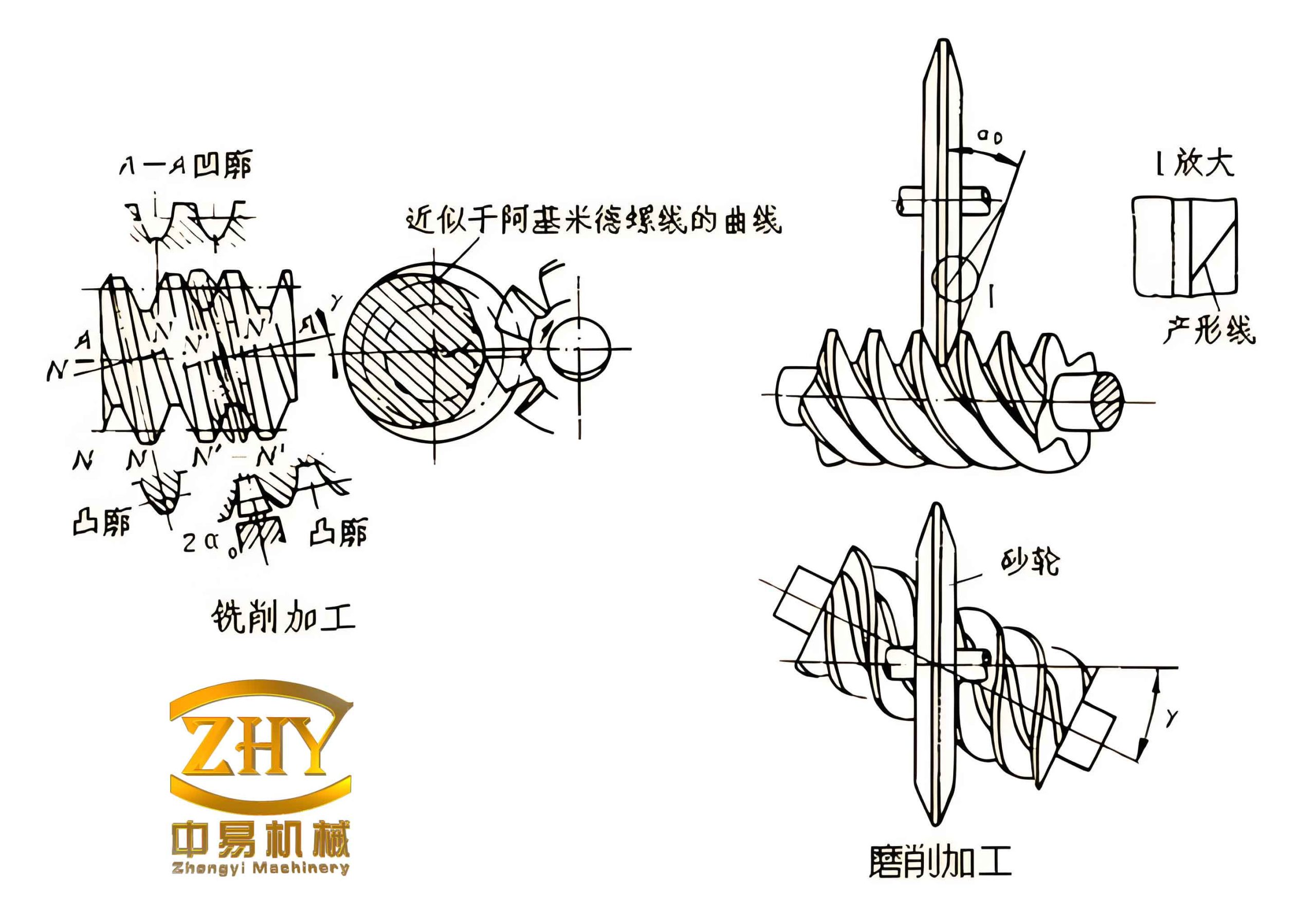
1. Calculation of Process Transmission Ratio for Machining Worms
1.1 The High-Order Modification Curve
To obtain a universal modification curve, I first transformed the measured modification data from reference literature into dimensionless form. For a worm drive with center distance \(a = 500\) mm and transmission ratio \(i_{12} = 8\), 35 sets of data points \((\varphi_x^{(i)}, \Delta_s^{(i)})\) were collected. I defined the angle coefficient:
$$ x = \frac{\varphi_x}{\varphi_w} = \frac{i_{12}\alpha – \varphi}{i_{12}\varphi_w} $$
where \(\varphi_w\) is the working half-angle of the worm enveloping the wheel. The modification amount coefficient is:
$$ I_i = \frac{\Delta_s^{(i)}}{\Delta_f} $$
where \(\Delta_f\) is the modification amount at the worm entrance, calculated as:
$$ \Delta_f = a\,(0.0003 + 0.000034\, i_{12}) \quad \text{(for } 10.25 \le i_{12} \le 59\text{)} $$
The dimensionless data after processing is shown in the table below:
| No. | Angle coefficient \(x\) | Modification coefficient \(I_i\) |
|---|---|---|
| 1 | 1.0000 | 1.0000 |
| 2 | 0.9412 | 0.9192 |
| 3 | 0.8824 | 0.8500 |
| … | … | … |
| 18 | 0 | 0.1000 |
| 19 | -0.0588 | 0.07692 |
| … | … | … |
| 35 | -1.0000 | 0.07692 |
Using the least squares method, I fitted the data to a polynomial of order \(n\):
$$ I_n(x) = \sum_{k=0}^{n} c_k x^k $$
The coefficients for different orders are listed below:
| Coefficient | 3rd order | 4th order | 5th order | 6th order | 7th order |
|---|---|---|---|---|---|
| \(c_0\) | 9.9857e-2 | 1.0202e-1 | 1.0202e-1 | 9.6396e-2 | 9.640e-2 |
| \(c_1\) | 5.0056e-1 | 5.0056e-1 | 5.2125e-1 | 5.2125e-1 | 5.1184e-1 |
| \(c_2\) | 4.2790e-1 | 4.0739e-1 | 4.0739e-1 | 5.2004e-1 | 5.2004e-1 |
| \(c_3\) | -4.5089e-2 | -4.5089e-2 | -1.3687e-1 | -1.3687e-1 | -5.5751e-2 |
| \(c_4\) | 0 | -2.2659e-2 | -2.2659e-2 | -2.9935e-1 | -2.9935e-1 |
| \(c_5\) | 0 | 0 | 7.8395e-2 | 7.8395e-2 | -9.2200e-2 |
| \(c_6\) | 0 | 0 | 0 | 2.2474e-1 | 2.2474e-1 |
| \(c_7\) | 0 | 0 | 0 | 0 | 1.0084e-1 |
The total fitting errors (sum of squared residuals) for different orders are:
| Order | 2 | 3 | 4 | 5 | 6 | 7 |
|---|---|---|---|---|---|---|
| Error | 6.9852e-2 | 5.4385e-2 | 5.3239e-2 | 4.9359e-2 | 3.9980e-2 | 3.9457e-2 |
The results show that simply increasing the polynomial order does not significantly improve the fitting accuracy. The modification curve is expressed as:
$$ \Delta = \Delta_f I_n(x) = \Delta_f \sum_{k=0}^{n} c_k x^k $$
When \(n=2\), it reduces to the parabolic modification curve; for \(n>2\), it becomes a high-order modification curve.
1.2 Relationship Between Process Transmission Ratio and Modification Curve
During the machining of the worm, the additional rotation of the tool \(\Delta\varphi_d\) is related to the change in modification amount. From the geometric relationship:
$$ \Delta\varphi_d = \frac{\Delta}{r_2} = \frac{\Delta_f}{r_2} I_n(x) $$
where \(r_2\) is the radius of the worm wheel pitch circle. The total tool rotation angle during machining is:
$$ \varphi_d = \frac{\varphi}{i_{12}} – \Delta\varphi_d = \frac{\varphi}{i_{12}} – \frac{\Delta_f}{r_2} I_n(x) $$
Differentiating with respect to \(\varphi\) gives the instantaneous process transmission ratio:
$$ i_{1d} = \frac{1}{d\varphi_d/d\varphi} = \frac{i_{12}}{1 + \frac{\Delta_f}{r_2\varphi_w} I’_n(x)} $$
where \(I’_n(x) = \sum_{k=1}^{n} k c_k x^{k-1}\). The sign of \(I’_n(x)\) determines whether \(i_{1d}\) is greater or less than the nominal ratio \(i_{12}\). In the modification curve, \(I’_n(x) = 0\) occurs near \(x \approx -0.5\). To the right of this point, \(I’_n(x) > 0\) and \(i_{1d} < i_{12}\); to the left, \(I’_n(x) < 0\) and \(i_{1d} > i_{12}\). This variable transmission ratio is the essence of the high-order modification.
2. Meshing Theory of High-Order Modified Globoidal Worm Drives
2.1 Coordinate Systems and Tool Edge Equation
The tooth surface of the straight profile globoidal worm is generated by a straight-edged lathe tool. I established a system of six coordinate systems: fixed systems \(\sigma_{o1}\), \(\sigma_{o2}\), \(\sigma_{od}\) attached to the frame, and moving systems \(\sigma_1\), \(\sigma_2\), \(\sigma_d\) attached to the worm, worm wheel, and tool respectively. The tool edge line is expressed in the tool coordinate system \(\sigma_d\) as:
$$ (\mathbf{r}_d)_d = -u\,\mathbf{i}_d + r_b\,\mathbf{j}_d $$
where \(u\) is the parameter along the cutting edge, and \(r_b\) is the base circle radius. After rotation by the process angle \(\varphi_d\), the family of tool lines in the auxiliary coordinate system \(\sigma_{od}\) is:
$$ (\mathbf{r}_d)_{od} = x_{od}\,\mathbf{i}_{od} + y_{od}\,\mathbf{j}_{od} $$
$$ x_{od} = -u\cos\varphi_d – r_b\sin\varphi_d, \quad y_{od} = -u\sin\varphi_d + r_b\cos\varphi_d $$
Transforming to the worm coordinate system \(\sigma_1\) yields:
$$ (\mathbf{r}_1)_1 = a\,\mathbf{R}[\mathbf{k}_1,-\varphi]\,\mathbf{i}_{o1} + \mathbf{R}[\mathbf{k}_1,-\varphi]\,\mathbf{R}[\mathbf{i}_{o1},\pi/2]\,(\mathbf{r}_d)_{od} $$
2.2 Proof of Non-Developability of the Worm Helical Surface
The worm helicoid can be written as a ruled surface:
$$ (\mathbf{r}_1)_1 = \boldsymbol{\rho}(\varphi) + u\,\mathbf{t}(\varphi) $$
where \(\boldsymbol{\rho}(\varphi)\) and \(\mathbf{t}(\varphi)\) are functions of \(\varphi\). Compute the derivatives:
$$ \boldsymbol{\rho}'(\varphi) = \mathbf{R}[\mathbf{k}_1,-\varphi]\,\mathbf{R}[\mathbf{i}_{o1},\pi/2]\,\mathbf{R}[\mathbf{k}_{od},\varphi_d] \left( -\frac{1}{i_{1d}}\mathbf{i}_d + (a – r_b\sin\varphi_d)\,\mathbf{k}_d \right) $$
$$ \mathbf{t}'(\varphi) = \mathbf{R}[\mathbf{k}_1,-\varphi]\,\mathbf{R}[\mathbf{i}_{o1},\pi/2]\,\mathbf{R}[\mathbf{k}_{od},\varphi_d] \left( -\frac{1}{i_{1d}}\mathbf{j}_d – \cos\varphi_d\,\mathbf{k}_d \right) $$
The scalar triple product is:
$$ [\boldsymbol{\rho}'(\varphi), \mathbf{t}(\varphi), \mathbf{t}'(\varphi)] = \frac{1}{i_{1d}}(a – r_b\sin\varphi_d) \neq 0 $$
Since the triple product is nonzero, the surface is non-developable. This matches the known property of straight profile globoidal worm gears: their helicoid cannot be developed into a plane, which complicates precision grinding.
2.3 First and Second Fundamental Forms, Curvature Parameters
From the parametric representation, I computed the first fundamental quantities:
$$ E = 1, \quad F = \frac{r_b}{i_{1d}}, \quad G = (x_{od}+a)^2 + \left(u^2 + \frac{r_b^2}{i_{1d}^2}\right) $$
The unit normal vector is:
$$ (\mathbf{n}_1)_1 = \frac{1}{D}\,\mathbf{R}[\mathbf{k}_1,-\varphi]\,\mathbf{R}[\mathbf{i}_{o1},\pi/2]\,\mathbf{R}[\mathbf{k}_{od},\varphi_d] \left[ (a+x_{od})\mathbf{j}_d + \frac{u}{i_{1d}}\mathbf{k}_d \right] $$
where \(D = \sqrt{(u/i_{1d})^2 + (a+x_{od})^2}\). The second fundamental quantities are:
$$ L = 0, \quad M = \frac{r_b\sin\varphi_d – a}{i_{1d}D}, \quad N = \frac{a+x_{od}}{D}\left[ (a+x_{od})\sin\varphi_d – u\frac{d^2\varphi_d}{d\varphi^2} – \frac{r_b}{i_{1d}^2} \right] – \frac{2u y_{od}}{i_{1d}^2 D} $$
where
$$ \frac{d^2\varphi_d}{d\varphi^2} = -\frac{\Delta_f}{r_2 i_{12}^2 \varphi_w^2}\sum_{k=2}^{n} k(k-1)c_k x^{k-2} $$
The normal curvature along the \(u\)-direction (direction \(\mathbf{t}(\varphi)\)) is zero:
$$ k_\xi = \frac{L}{E} = 0 $$
The geodesic torsion is:
$$ \tau_\xi = \frac{M}{D} $$
The mean curvature is:
$$ H = \frac{N – 2FM}{2D^2} $$
2.4 Worm Wheel Tooth Surface and Meshing Function
Assuming the worm angular velocity \(|\boldsymbol{\omega}_1| = 1\) rad/s, the relative angular velocity is:
$$ (\boldsymbol{\omega}_{12})_{o1} = \frac{1}{i_{12}}\mathbf{j}_{o1} + \mathbf{k}_{o1} $$
The family of worm surfaces in \(\sigma_{o1}\) is obtained by rotation:
$$ (\mathbf{r}_1^*)_{o1} = \mathbf{R}[\mathbf{k}_{o1},\varphi_1]\,(\mathbf{r}_1)_1 $$
$$ (\mathbf{n}_1^*)_{o1} = \mathbf{R}[\mathbf{k}_{o1},\varphi_1]\,(\mathbf{n}_1)_1 $$
The relative velocity vector is:
$$ (\mathbf{V}_{12})_{o1} = \left( \frac{y_{od}}{i_{12}} – (x_{od}+a)\sin(\varphi_1-\varphi) \right)\mathbf{i}_{o1} + (x_{od}+a)\cos(\varphi_1-\varphi)\,\mathbf{j}_{o1} – \frac{1}{i_{12}}\mathbf{k}_{o1} $$
The meshing function \(\Phi\) is derived from \(\Phi = (\mathbf{n}_1^*)_{o1}\cdot(\mathbf{V}_{12})_{o1} = 0\):
$$ \Phi(u,\varphi,\varphi_1) = \frac{1}{i_{12}D}\left[A\sin(\varphi_1-\varphi) + B\cos(\varphi_1-\varphi) + C\right] = 0 $$
with
$$ A = \frac{u y_{od}}{i_{1d}}, \quad B = (x_{od}+a)(u – a\cos\varphi_d), \quad C = (x_{od}+a)\left(a\cos\varphi_d – \frac{i_{12}}{i_{1d}}u\right) $$
Solving \(\Phi=0\) yields two solutions \(\varphi_{1A}\) and \(\varphi_{1B}\) corresponding to two sub-conjugate zones \(\Sigma_A\) and \(\Sigma_B\) on the worm wheel tooth surface. The wheel tooth surface equation in \(\sigma_2\) is:
$$ (\mathbf{r}_2)_2 = \mathbf{R}[\mathbf{k}_2, -\varphi_1/i_{12}] \left\{ \mathbf{R}[\mathbf{i}_{o2}, -\pi/2]\,(\mathbf{r}_1^*)_{o1} – a\mathbf{i}_{o2} \right\} $$
with components:
$$ x_2 = [(x_{od}+a)\cos(\varphi_1-\varphi)-a]\cos(\varphi_1/i_{12}) + y_{od}\sin(\varphi_1/i_{12}) $$
$$ y_2 = [a-(x_{od}+a)\cos(\varphi_1-\varphi)]\sin(\varphi_1/i_{12}) + y_{od}\cos(\varphi_1/i_{12}) $$
$$ z_2 = -(x_{od}+a)\sin(\varphi_1-\varphi) $$
2.5 Curvature Interference Boundary and Induced Normal Curvature
The derivative of the meshing function with respect to \(\varphi_1\) is:
$$ \Phi_{\varphi_1} = \frac{1}{i_{12}D}[A\cos(\varphi_1-\varphi) – B\sin(\varphi_1-\varphi)] $$
The normal vector to the instantaneous contact line is:
$$ (\mathbf{N})_{o1} = N_\xi (\boldsymbol{\alpha}_\xi)_{o1} + N_\eta (\boldsymbol{\alpha}_\eta)_{o1} $$
where
$$ N_\xi = \tau_\xi (\mathbf{V}_{12})_{o1}\cdot(\boldsymbol{\alpha}_\eta)_{o1} + (\boldsymbol{\omega}_{12})_{o1}\cdot(\boldsymbol{\alpha}_\eta)_{o1} $$
$$ N_\eta = 2H (\mathbf{V}_{12})_{o1}\cdot(\boldsymbol{\alpha}_\eta)_{o1} + \tau_\xi (\mathbf{V}_{12})_{o1}\cdot(\boldsymbol{\alpha}_\xi)_{o1} – (\boldsymbol{\omega}_{12})_{o1}\cdot(\boldsymbol{\alpha}_\xi)_{o1} $$
The scalar products are calculated analytically. The curvature interference function is:
$$ \Psi = N_\xi (\mathbf{V}_{12})_{o1}\cdot(\boldsymbol{\alpha}_\xi)_{o1} + N_\eta (\mathbf{V}_{12})_{o1}\cdot(\boldsymbol{\alpha}_\eta)_{o1} + \Phi_{\varphi_1} $$
When \(\Psi = 0\), curvature interference occurs. The induced normal curvature and sliding angle are:
$$ k_N^{(12)} = \frac{N_\xi^2 + N_\eta^2}{\Psi} $$
$$ \theta_{vt} = \arcsin\!\left( \frac{|\Psi – \Phi_{\varphi_1}|}{|\mathbf{V}_{12}|_{o1}\sqrt{N_\xi^2+N_\eta^2}} \right) $$
3. Numerical Examples and Analysis
I performed numerical simulations for a worm drive with parameters: worm threads \(Z_1=2\), center distance \(a=280\) mm, transmission ratio \(i_{12}=25\). The calculated geometric parameters are listed in the table below.
| Parameter | Formula | Value |
|---|---|---|
| Worm pitch diameter \(d_1\) | \(0.681a^{0.875}\) | 94 mm |
| Worm wheel pitch diameter \(d_2\) | \(2a-d_1\) | 466 mm |
| Worm wheel face width \(b_2\) | \(0.25a\) | 70 mm |
| Base circle diameter \(d_b\) | \(0.625a\) | 175 mm |
| Pressure angle \(\alpha\) | \(\arcsin(d_b/d_2)\) | 22.0589° |
| Number of wheel teeth \(Z_2\) | \(i_{12}Z_1\) | 50 |
| Transverse module \(m_t\) | \(d_2/Z_2\) | 9.3200 mm |
| Number of worm enveloped teeth \(Z_k\) | \(Z_2/10\) | 5 |
| Working half-angle \(\varphi_w\) | \(\pi(Z_k-0.5)/Z_2\) | 16.3809° |
| Worm working length \(L_w\) | \(d_2\sin\varphi_w\) | 131.4151 mm |
| Worm addendum diameter \(d_{a1}\) | \(d_1+1.5m_t\) | 107.98 mm |
| Worm wheel addendum diameter \(d_{a2}\) | \(d_2+1.5m_t\) | 479.98 mm |
| Worm wheel max. addendum diameter \(d_{ea2}\) | \(d_{a2}+m_t\) | 489 mm |
| Worm addendum arc radius \(R_{a1}\) | \(a-0.5d_{a1}\) | 226.0100 mm |
| Worm wheel addendum arc radius \(R_{a2}\) | \(\ge 0.53(d_{a1}-3.4m_t)\) | 41 mm |
| Worm wheel root arc radius \(R_{f2}\) | \(0.5d_{a1}+0.2m_t\) | 55.8540 mm |
| Entrance modification \(\Delta_f\) | Eq. (3) | 0.3239 mm |
| Speed ratio correction range (3rd order) | \(\Delta i = i_{1d}-i_{12}\) | [-0.1479, 0.0704] |
| Speed ratio correction range (4th order) | [-0.1539, 0.0787] | |
| Speed ratio correction range (5th order) | [-0.1708, 0.0510] | |
| Speed ratio correction range (6th order) | [-0.2062, 0.1226] | |
| Speed ratio correction range (7th order) | [-0.2169, 0.0949] |
3.1 Meshing Characteristics of the Original (Unmodified) Drive
For the original drive, I set \(i_{1d}=i_{12}\). The conjugate zones on the worm and wheel surfaces were computed. On the worm surface, the sub-conjugate zone \(\Sigma_A\) degenerates into a single constant contact line. On the wheel surface, zone \(\Sigma_A\) is a line, while zone \(\Sigma_B\) occupies a finite region bounded by the engagement boundary and a curvature interference line. The induced normal curvature and sliding angle were evaluated at three sampling points (a: intersection of contact line with worm wheel addendum, b: with worm pitch circle, c: with worm addendum).
| Contact line index | Point a: \(k_N^{(12)}\) (mm⁻¹) | Point a: \(\theta_{vt}\) (°) | Point b: \(k_N^{(12)}\) (mm⁻¹) | Point b: \(\theta_{vt}\) (°) | Point c: \(k_N^{(12)}\) (mm⁻¹) | Point c: \(\theta_{vt}\) (°) |
|---|---|---|---|---|---|---|
| 1′ | 0.0065 | 47.96 | 0.0049 | 54.78 | 0.0039 | 60.41 |
| 2′ | 0.0052 | 53.16 | 0.0039 | 59.79 | 0.0032 | 64.93 |
| 3′ | 0.0032 | 61.03 | 0.0026 | 66.51 | 0.0022 | 70.61 |
| 4′ | 0.0013 | 73.52 | 0.0012 | 76.20 | 0.0011 | 78.19 |
| 5′ | 0.0000 | 0/0 | 0.0001 | 89.23 | 0.0002 | 88.78 |
The original drive shows excellent lubrication conditions in \(\Sigma_B\) (low \(k_N\) and high \(\theta_{vt}\)), but the constant contact line in \(\Sigma_A\) makes it prone to early failure.
3.2 High-Order Modified Drives
I analyzed three cases: 3rd order, 5th order, and 7th order modification curves. For each, the conjugate zones on the worm and wheel surfaces were plotted. The results show that the constant contact line is eliminated, and zone \(\Sigma_A\) becomes a finite region. However, a curvature interference boundary (where \(\Psi=0\)) appears inside \(\Sigma_A\), limiting the usable area. On the wheel surface, zone \(\Sigma_B\) extends to the worm exit end, indicating full-length utilization of the worm.
Higher-order modification (e.g., 7th) further enlarges \(\Sigma_A\) and reduces the curvature interference line length. At the intersection of the curvature interference boundary with the worm addendum, a part of the tooth can be trimmed to avoid interference. The meshing quality parameters are summarized below.
| Contact line | Point a: \(k_N^{(12)}\) (mm⁻¹) | Point a: \(\theta_{vt}\) (°) | Point b: \(k_N^{(12)}\) (mm⁻¹) | Point b: \(\theta_{vt}\) (°) | Point c: \(k_N^{(12)}\) (mm⁻¹) | Point c: \(\theta_{vt}\) (°) |
|---|---|---|---|---|---|---|
| 1 (in \(\Sigma_A\)) | 0.1170 | 83.46 | 0.0747 | 84.67 | 0.0498 | 85.79 |
| 1′ | 0.0076 | 50.98 | 0.0066 | 56.10 | 0.0059 | 61.40 |
| 2′ | 0.0056 | 61.67 | 0.0052 | 66.73 | 0.0050 | 70.33 |
| 3′ | 0.0026 | 83.95 | 0.0027 | 83.06 | 0.0028 | 82.63 |
| 4′ | 0.0069 | 86.49 | 0.0033 | 87.42 | 0.0018 | 88.20 |
| 5′ | 0.0155 | 83.15 | 0.0086 | 82.41 | 0.0047 | 80.61 |
| Contact line | Point a: \(k_N^{(12)}\) (mm⁻¹) | Point a: \(\theta_{vt}\) (°) | Point b: \(k_N^{(12)}\) (mm⁻¹) | Point b: \(\theta_{vt}\) (°) | Point c: \(k_N^{(12)}\) (mm⁻¹) | Point c: \(\theta_{vt}\) (°) |
|---|---|---|---|---|---|---|
| 1 | 0.0388 | 83.47 | 0.0264 | 84.73 | 0.0191 | 85.88 |
| 1′ | 0.0066 | 51.51 | 0.0056 | 56.33 | 0.0048 | 61.53 |
| 2′ | 0.0055 | 61.70 | 0.0051 | 66.78 | 0.0049 | 70.38 |
| 3′ | 0.0027 | 83.85 | 0.0028 | 82.96 | 0.0029 | 82.54 |
| 4′ | 0.0063 | 86.39 | 0.0030 | 87.30 | 0.0016 | 88.08 |
| 5′ | 0.0339 | 83.43 | 0.0212 | 82.83 | 0.0140 | 81.34 |
| Contact line | Point a: \(k_N^{(12)}\) (mm⁻¹) | Point a: \(\theta_{vt}\) (°) | Point b: \(k_N^{(12)}\) (mm⁻¹) | Point b: \(\theta_{vt}\) (°) | Point c: \(k_N^{(12)}\) (mm⁻¹) | Point c: \(\theta_{vt}\) (°) |
|---|---|---|---|---|---|---|
| 1 | 0.0144 | 83.42 | 0.0102 | 84.67 | 0.0077 | 85.81 |
| 1′ | 0.0047 | 55.29 | 0.0039 | 59.47 | 0.0031 | 64.38 |
| 2′ | 0.0060 | 63.22 | 0.0057 | 68.29 | 0.0057 | 71.90 |
| 3′ | 0.0025 | 83.83 | 0.0026 | 83.32 | 0.0026 | 83.09 |
| 4′ | 0.0079 | 77.89 | 0.0038 | 81.63 | 0.0020 | 84.07 |
| 5′ | 0.0092 | 78.72 | 0.0049 | 70.97 | 0.0025 | 73.12 |
The tables show that high-order modification does not significantly degrade the local meshing quality: the induced normal curvature remains low, and the sliding angle remains high, ensuring good lubrication. However, the presence of the curvature interference boundary in zone \(\Sigma_A\) is a drawback. By increasing the polynomial order, the length of the interference boundary can be reduced but not completely eliminated. For the 7th-order case, a portion of the interference line near the wheel root can be trimmed away by intersecting with the exit boundary.
4. Conclusion
In this work, I established a comprehensive mathematical model for straight profile globoidal worm gears with high-order modification. By normalizing the modification data from natural wear measurements and fitting them with high-order polynomials, I derived a universal modification curve. The process transmission ratio \(i_{1d}\) was then expressed as a function of this curve, which allowed me to incorporate the modification effect directly into the meshing analysis. I proved rigorously that the helicoid of the straight profile globoidal worm is a non-developable ruled surface, which is consistent with its generation principle.
Numerical simulations demonstrated that high-order modification successfully eliminates the constant contact line that plagues the original drive. The conjugate zone on the worm wheel tooth surface expands significantly, and the full length of the worm is engaged in meshing. At the worm entrance, a portion of double-line contact is preserved, enhancing load capacity. The induced normal curvature and sliding angle remain favorable, indicating good lubrication conditions.
Nevertheless, a curvature interference boundary appears within zone \(\Sigma_A\) on the worm wheel tooth surface, which may lead to undercutting if not properly managed. Increasing the polynomial order of the modification curve reduces the extent of this interference but cannot remove it entirely. Given the complexity of implementing variable transmission ratio machining in practice, and the persistent issue of curvature interference, high-order modification alone is not recommended as a standalone strategy. It should be combined with other rational modification parameters (e.g., offset distance, center distance variation) to achieve optimal performance.
In summary, my study provides a complete theoretical foundation for the design and analysis of high-order modified straight profile globoidal worm gears, offering valuable insights into how to balance contact pattern enlargement and interference avoidance.