
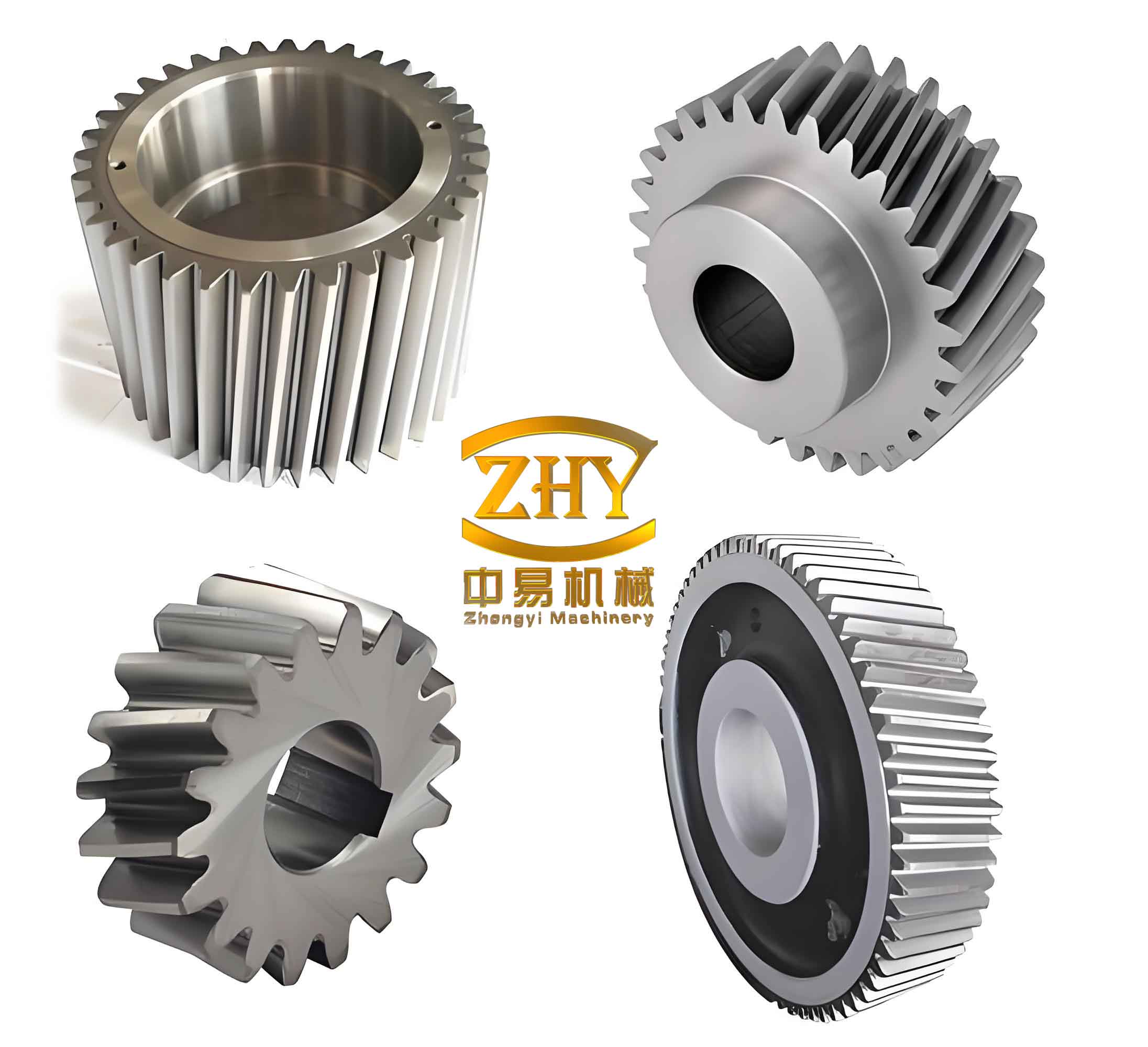
In my research, I study a design method for high power density asymmetric helical gear transmissions used in electric vehicle drivetrains. The central problem is simple to state but difficult to solve: an electric vehicle reducer must transmit a large torque within a very small space, while the forward driving condition and the forward reverse-drag condition have different life requirements. A conventional symmetric helical gear uses the same pressure angle on both flanks, so increasing the pressure angle improves contact strength and bending strength but also thins the tooth tip. This trade-off limits the achievable power density. I therefore investigate an asymmetric helical gear pair with two different pressure angles, one for the driving flank and one for the reverse-drag flank. By making the driving flank pressure angle larger and the reverse-drag flank pressure angle smaller, I can balance the safety margins of the two flanks and reduce the gear pair volume under the same torque. I also address the vibration excitation caused by high rotational speed, because electric vehicle motors often operate above 12000 rpm, and loaded transmission error is one of the most important excitations for gear whine and vibration. My method combines tooth surface generation, geometric contact analysis, loaded contact analysis, macro-geometry optimization, and micro-modification optimization. I validate the proposed method with a professional gear transmission software package.
The first step in my method is to generate an accurate asymmetric involute helical gear tooth surface. I use a rack cutter with two different pressure angles. The rack cutter is simple, manufacturable, and compatible with common gear cutting machines. I define the normal module as \(m_n\), the helix angle as \(\beta\), the number of teeth as \(z\), the profile shift coefficient as \(x_n\), the normal pressure angle on the driving flank as \(\alpha_{n1}\), and the normal pressure angle on the reverse-drag flank as \(\alpha_{n2}\). The rack cutter generates the gear tooth surface through pure rolling between the pitch line of the rack and the pitch circle of the helical gear. Because the two flanks have different pressure angles, the generating process is asymmetric, and the resulting helical gear has a non-symmetric tooth profile.
To describe the generation process mathematically, I use several coordinate systems. The coordinate system \(S_a\) is fixed to the rack cutter. The coordinate system \(S_b\) is an auxiliary system fixed to the rack. The coordinate system \(S_i\) is fixed to the generated helical gear. The fixed coordinate system \(S_f\) is used to relate the rack translation and the gear rotation. The rack displacement is \(r_p \theta\), and the gear rotation is \(\theta\), where \(r_p\) is the pitch radius. The profile shift produces an additional displacement \(x_n m_n\). The transformation from the rack cutter coordinate system to the gear coordinate system can be written as
$$
\mathbf{M}_{ib} =
\begin{bmatrix}
\cos\theta & \sin\theta & 0 & (r_p + x_n m_n)\cos\theta + r_p\theta \sin\theta \\
-\sin\theta & \cos\theta & 0 & -(r_p + x_n m_n)\sin\theta + r_p\theta \cos\theta \\
0 & 0 & 1 & 0 \\
0 & 0 & 0 & 1
\end{bmatrix}.
$$
For the involute portion of the rack cutter, I describe the two flanks by independent parameters \(l_j\) and \(u_j\), where \(j=1\) corresponds to the driving flank and \(j=2\) corresponds to the reverse-drag flank. The position vector of the rack cutter in its local coordinate system is
$$
\mathbf{R}_{j}(l_j,u_j) =
\begin{bmatrix}
x_j(l_j,u_j) \\
y_j(l_j,u_j) \\
z_j(l_j,u_j)
\end{bmatrix}.
$$
The corresponding unit normal vector is obtained from the cross product of the partial derivatives:
$$
\mathbf{n}_{j} =
\frac{
\frac{\partial \mathbf{R}_{j}}{\partial l_j}
\times
\frac{\partial \mathbf{R}_{j}}{\partial u_j}
}{
\left|
\frac{\partial \mathbf{R}_{j}}{\partial l_j}
\times
\frac{\partial \mathbf{R}_{j}}{\partial u_j}
\right|
}.
$$
After transforming the rack cutter surface into the gear coordinate system, the generated tooth surface of the asymmetric helical gear must satisfy the meshing equation. For the involute flank, the meshing equation is
$$
f_i = n_{bjx}(R_{bjy} – r_p\theta) – n_{bjy}(R_{bjx} + x_n m_n) = 0.
$$
For the fillet or transition portion generated by the rack cutter tip, the meshing equation includes the relative velocity:
$$
f_{sj} = \mathbf{n}_{sj} \cdot \mathbf{v}_{12} = 0.
$$
The relative velocity \(\mathbf{v}_{12}\) is computed from the rack velocity and the gear rotation:
$$
\mathbf{v}_{12} =
\begin{bmatrix}
0 \\
0 \\
1
\end{bmatrix}
\times
\mathbf{R}_{fsj}
–
\begin{bmatrix}
0 \\
0 \\
\omega
\end{bmatrix}
\times
\mathbf{R}_{fsj}.
$$
Using these equations, I generate the complete asymmetric helical gear tooth surface. The driving flank and the reverse-drag flank are generated separately because they have different pressure angles. The transition fillet is generated by the rack cutter tip radius \(\rho\). The final tooth surface is smooth and accurate, and it forms the basis for all subsequent contact and stress analyses. The main geometric parameters I use in the initial electric vehicle helical gear pair are listed in Table 1.
| Parameter | Symbol | Initial value |
|---|---|---|
| Normal module | \(m_n\) | 1.88 mm |
| Number of teeth of pinion | \(z_1\) | 26 |
| Number of teeth of wheel | \(z_2\) | 75 |
| Driving flank pressure angle | \(\alpha_{n1}\) | 20° |
| Reverse-drag flank pressure angle | \(\alpha_{n2}\) | 20° |
| Helix angle | \(\beta\) | 21.5° |
| Face width | \(b\) | 30 mm |
| Addendum | \(h_a\) | 1.88 mm |
| Dedendum | \(h_f\) | 2.35 mm |
| Pinion profile shift | \(x_{n1}\) | 0.051 |
| Wheel profile shift | \(x_{n2}\) | -0.062 |
After generating the tooth surface, I build a geometric contact analysis model, commonly called TCA. The TCA model determines the contact path, the contact ellipse, and the geometric transmission error under light load. For an asymmetric helical gear pair, the two tooth surfaces must have a common contact point and a common normal at every instant. In the fixed coordinate system \(S_f\), the contact condition can be written as
$$
\mathbf{R}_{f1}(u_1,l_1,\phi_1) = \mathbf{R}_{f2}(u_2,l_2,\phi_2),
$$
$$
\mathbf{n}_{f1}(u_1,l_1,\phi_1) = \mathbf{n}_{f2}(u_2,l_2,\phi_2).
$$
Here, \(\phi_1\) and \(\phi_2\) are the rotation angles of the pinion and the wheel. The transformation from the pinion coordinate system to the fixed coordinate system includes the center distance \(E\) and the pinion rotation. The transformation from the wheel coordinate system to the fixed coordinate system includes the wheel rotation, the horizontal axis installation error \(\Delta\delta\), and the vertical axis installation error \(\Delta\varepsilon\). The corresponding transformation matrices are
$$
\mathbf{M}_{f1} =
\begin{bmatrix}
\cos\phi_1 & \sin\phi_1 & 0 & E \\
-\sin\phi_1 & \cos\phi_1 & 0 & 0 \\
0 & 0 & 1 & 0 \\
0 & 0 & 0 & 1
\end{bmatrix},
$$
$$
\mathbf{M}_{f2} =
\mathbf{M}_{fh2}\mathbf{M}_{h2}.
$$
The installation error matrix is
$$
\mathbf{M}_{h2} =
\begin{bmatrix}
1 & 0 & 0 & 0 \\
0 & \cos\Delta\delta & \sin\Delta\delta & 0 \\
0 & -\sin\Delta\delta & \cos\Delta\delta & 0 \\
0 & 0 & 0 & 1
\end{bmatrix}
\begin{bmatrix}
\cos\Delta\varepsilon & 0 & \sin\Delta\varepsilon & 0 \\
0 & 1 & 0 & 0 \\
-\sin\Delta\varepsilon & 0 & \cos\Delta\varepsilon & 0 \\
0 & 0 & 0 & 1
\end{bmatrix}.
$$
By solving the TCA equations for a series of pinion rotation angles, I obtain the contact path on both the pinion and the wheel. The geometric transmission error is calculated as
$$
\Delta\phi_2 = (\phi_2 – \phi_{20}) – \frac{z_1}{z_2}(\phi_1 – \phi_{10}),
$$
where \(\phi_{10}\) and \(\phi_{20}\) are the initial rotation angles. The geometric transmission error describes the deviation from a perfectly conjugate motion. A small transmission error fluctuation is desirable because it indicates smooth meshing. However, the TCA model alone does not include the effect of load. Therefore, I also develop a loaded contact analysis model, LTCA.
The LTCA model is based on the TCA results and includes the flexibility of the gear teeth. I discretize the contact line into a set of points. For each point \(q\), the load intensity is \(p_q\), the deformation is \(d_q\), and the initial gap is \(w_q\). The flexibility matrix \(\mathbf{F}\) relates the load to the deformation. The deformation compatibility equation can be written as
$$
\mathbf{F}\mathbf{p} + \mathbf{w} + \mathbf{d} = \mathbf{Z},
$$
where \(\mathbf{Z}\) is the rigid body displacement vector. The load balance condition is
$$
\sum_{q=1}^{2n+1} p_q = P.
$$
The contact condition requires that if a point is in contact, then its gap is zero and its load is positive; if a point is not in contact, then its gap is positive and its load is zero. This can be expressed as
$$
p_q > 0 \Rightarrow d_q = 0,
$$
$$
p_q = 0 \Rightarrow d_q > 0.
$$
The LTCA problem is solved as a mathematical programming problem. The objective is to minimize the total deformation energy:
$$
\min \quad \mathbf{p}^T \mathbf{F} \mathbf{p} + \mathbf{p}^T \mathbf{w} + \mathbf{p}^T \mathbf{d}.
$$
Subject to the load balance condition and the contact boundary conditions, I solve for the load distribution, the loaded transmission error, the contact stress, and the root bending stress. The maximum contact stress in the contact ellipse is calculated from Hertzian theory:
$$
\sigma_H = \frac{3P_c}{2\pi a_c b_c},
$$
where \(a_c\) and \(b_c\) are the semi-major and semi-minor axes of the contact ellipse. These axes are obtained from the principal curvatures of the two contacting tooth surfaces. If the principal curvatures of the pinion are \(k_f\) and \(k_h\), and those of the wheel are \(k_s\) and \(k_q\), then the geometric parameters of the contact ellipse are
$$
A_c = \frac{1}{2}\left(k_f + k_h + k_s + k_q\right),
$$
$$
B_c = \frac{1}{2}\left[
\left(k_f – k_h\right)^2 +
\left(k_s – k_q\right)^2 +
2\left(k_f – k_h\right)\left(k_s – k_q\right)\cos 2\sigma
\right]^{1/2}.
$$
The semi-axes are
$$
a_c = \alpha_c \left[
\frac{3P_c}{4}\left(
\frac{1-\mu_1^2}{E_1} + \frac{1-\mu_2^2}{E_2}
\right)
\right]^{1/3} A_c^{-1/3},
$$
$$
b_c = \beta_c \left[
\frac{3P_c}{4}\left(
\frac{1-\mu_1^2}{E_1} + \frac{1-\mu_2^2}{E_2}
\right)
\right]^{1/3} B_c^{-1/3}.
$$
For the bending stress at the tooth root, I use an influence matrix method. First, I apply a unit normal load at each tooth surface node and compute the induced stress field. This gives a stress influence matrix \(\mathbf{S}\). Then I combine it with the load distribution vector \(\mathbf{L}\) obtained from LTCA:
$$
\boldsymbol{\sigma}_F = \mathbf{S} \mathbf{L}.
$$
Using the fourth strength theory, I compute the equivalent stress. This procedure allows me to evaluate the root bending stress of the asymmetric helical gear under various loads and installation errors.
Before optimizing the macro geometry, I analyze the sensitivity of the asymmetric helical gear to installation errors. The installation errors include the horizontal axis error \(\Delta\delta\) and the vertical axis error \(\Delta\varepsilon\). For a proper contact pattern, the contact trace should cover more than 80% of the tooth height and remain within the tooth surface. I calculate the allowable installation error range for different driving flank pressure angles. The results are shown in Table 2.
| Driving flank pressure angle \(\alpha_{n1}\) | Error type | Error range | Allowable tolerance |
|---|---|---|---|
| 15° | \(\Delta\delta\) | [-0.042°, 0.044°] | 0.086° |
| 15° | \(\Delta\varepsilon\) | [-0.013°, 0.012°] | 0.025° |
| 17.5° | \(\Delta\delta\) | [-0.048°, 0.045°] | 0.093° |
| 17.5° | \(\Delta\varepsilon\) | [-0.016°, 0.015°] | 0.031° |
| 20° | \(\Delta\delta\) | [-0.044°, 0.047°] | 0.092° |
| 20° | \(\Delta\varepsilon\) | [-0.019°, 0.018°] | 0.037° |
| 22.5° | \(\Delta\delta\) | [-0.052°, 0.049°] | 0.101° |
| 22.5° | \(\Delta\varepsilon\) | [-0.025°, 0.021°] | 0.046° |
| 25° | \(\Delta\delta\) | [-0.051°, 0.050°] | 0.101° |
| 25° | \(\Delta\varepsilon\) | [-0.025°, 0.025°] | 0.050° |
I observe that as the driving flank pressure angle increases, the allowable installation error tolerance becomes larger. This means that a larger pressure angle makes the asymmetric helical gear less sensitive to installation errors. Since the driving condition of an electric vehicle usually involves higher speed and higher load than the reverse-drag condition, increasing the driving flank pressure angle is beneficial. It improves the contact strength and also reduces the sensitivity to installation errors.
Next, I analyze the influence of macro geometry parameters on the contact stress and root bending stress of the asymmetric helical gear. I keep all other parameters constant and vary one parameter at a time. The results for the driving wheel bending stress under different pressure angle combinations are shown in Table 3. The pressure angle on the driving flank is denoted by \(\alpha_{n1}\), and the pressure angle on the reverse-drag flank is denoted by \(\alpha_{n2}\).
| \(\alpha_{n1}\) | \(\alpha_{n2}=15^\circ\) | \(\alpha_{n2}=17.5^\circ\) | \(\alpha_{n2}=20^\circ\) | \(\alpha_{n2}=22.5^\circ\) | \(\alpha_{n2}=25^\circ\) |
|---|---|---|---|---|---|
| 17.5° | 383.0 MPa | 359.6 MPa | 340.3 MPa | 327.6 MPa | 314.4 MPa |
| 20° | 413.9 MPa | 398.7 MPa | 376.5 MPa | 362.5 MPa | 348.4 MPa |
| 22.5° | 439.0 MPa | 415.1 MPa | 391.4 MPa | 370.9 MPa | 360.3 MPa |
The results show that when the reverse-drag flank pressure angle increases, the driving flank bending stress decreases. However, when the driving flank pressure angle increases while the reverse-drag flank pressure angle is fixed, the driving flank bending stress increases. This indicates that the two pressure angles must be selected carefully. A larger driving flank pressure angle improves contact strength but may increase bending stress. A larger reverse-drag flank pressure angle can reduce bending stress but may reduce reverse-drag contact strength. Therefore, I need an optimization model to find a balanced design.
I also study the effect of the normal module, helix angle, and number of teeth. The results are summarized in Table 4 and Table 5. In general, increasing the normal module, helix angle, and number of teeth reduces both contact stress and bending stress. However, increasing these parameters also increases the center distance or the gear volume, which reduces the power density. Therefore, the optimization must consider both strength and volume.
| Pressure angle pair | \(m_n=1.5\) mm | \(m_n=1.75\) mm | \(m_n=2.0\) mm | \(m_n=2.25\) mm | \(m_n=2.5\) mm |
|---|---|---|---|---|---|
| 20°/17.5° | 865.7 MPa | 416.4 MPa | 393.5 MPa | 257.0 MPa | 234.0 MPa |
| 20°/20° | 815.7 MPa | 392.7 MPa | 372.0 MPa | 243.2 MPa | 220.2 MPa |
| 20°/22.5° | 775.8 MPa | 379.5 MPa | 357.6 MPa | 232.2 MPa | 208.2 MPa |
| Pressure angle pair | \(\beta=18^\circ\) | \(\beta=19^\circ\) | \(\beta=20^\circ\) | \(\beta=21^\circ\) | \(\beta=22^\circ\) |
|---|---|---|---|---|---|
| 20°/17.5° | 810.5 MPa | 408.1 MPa | 405.2 MPa | 371.7 MPa | 369.4 MPa |
| 20°/20° | 767.1 MPa | 384.0 MPa | 379.4 MPa | 350.1 MPa | 348.0 MPa |
| 20°/22.5° | 738.4 MPa | 371.7 MPa | 351.4 MPa | 338.6 MPa | 333.2 MPa |
Based on these trends, I formulate a macro-geometry optimization model for the high power density asymmetric helical gear. The optimization variables are the driving flank pressure angle \(\alpha_{n1}\), the reverse-drag flank pressure angle \(\alpha_{n2}\), the pinion tooth number \(z_1\), the wheel tooth number \(z_2\), the normal module \(m_n\), and the helix angle \(\beta\). The objective is to minimize the center distance, which directly reflects the power density for a given torque and speed. The constraints include contact stress limits, bending stress limits, tip thickness limits, and no-undercut conditions. The optimization model can be written as
$$
\min_{\mathbf{X}} \quad a(\mathbf{X}) = \frac{m_n (z_1+z_2)}{2\cos\beta},
$$
subject to
$$
F_{H1}(\mathbf{X}) \le F_{H,\text{lim},1}, \quad F_{H2}(\mathbf{X}) \le F_{H,\text{lim},2},
$$
$$
F_{F1}(\mathbf{X}) \le F_{F,\text{lim},1}, \quad F_{F2}(\mathbf{X}) \le F_{F,\text{lim},2},
$$
$$
S_{a1}(\mathbf{X}) \ge 0.4 m_n, \quad S_{a2}(\mathbf{X}) \ge 0.4 m_n,
$$
$$
g_1(\mathbf{X}) \ge 0, \quad g_2(\mathbf{X}) \ge 0,
$$
$$
20^\circ \le \alpha_{n1} \le 24^\circ, \quad 16^\circ \le \alpha_{n2} \le 20^\circ,
$$
$$
40 \le z_1 \le 65, \quad 80 \le z_2 \le 100,
$$
$$
1.5 \le m_n \le 2.5, \quad 20^\circ \le \beta \le 30^\circ.
$$
The optimization vector is
$$
\mathbf{X} = [\alpha_{n1}, \alpha_{n2}, z_1, z_2, m_n, \beta]^T.
$$
I use a genetic algorithm to solve this optimization problem. The genetic algorithm is suitable because the objective function and constraints are highly nonlinear, and the contact and stress analyses are computationally expensive. The control parameters I use are listed in Table 6.
| Genetic algorithm parameter | Value |
|---|---|
| Population size | 20 |
| Crossover probability | 0.9 |
| Mutation probability | 0.05 |
| Maximum generations | 60 |
After optimization, the geometric parameters of the asymmetric helical gear pair are obtained. The comparison before and after optimization is shown in Table 7. The power density improvement is shown in Table 8.
| Parameter | Before optimization | After optimization |
|---|---|---|
| Pinion tooth number \(z_1\) | 26 | 23 |
| Wheel tooth number \(z_2\) | 75 | 69 |
| Normal module \(m_n\) | 1.88 mm | 1.944 mm |
| Driving flank pressure angle \(\alpha_{n1}\) | 20° | 21.483° |
| Reverse-drag flank pressure angle \(\alpha_{n2}\) | 20° | 18.855° |
| Helix angle \(\beta\) | 21.5° | 23.85° |
| Addendum \(h_a\) | 1.88 mm | 1.944 mm |
| Dedendum \(h_f\) | 2.35 mm | 2.43 mm |
| Face width \(b\) | 30 mm | 30 mm |
| Pinion profile shift \(x_{n1}\) | 0.051 | 0.051 |
| Wheel profile shift \(x_{n2}\) | -0.062 | -0.062 |
| Result | Before optimization | After optimization | Change |
|---|---|---|---|
| Driving flank contact stress | 1342.1 MPa | 1177.1 MPa | -12.29% |
| Driving flank pinion bending stress | 376.5 MPa | 351.9 MPa | -6.53% |
| Driving flank wheel bending stress | 355.3 MPa | 355.9 MPa | +0.17% |
| Reverse-drag flank contact stress | 1342.1 MPa | 1466.2 MPa | +9.25% |
| Transmission power density | 41464 kW/m³ | 44656 kW/m³ | +7.65% |
The optimized asymmetric helical gear has a higher power density while satisfying the strength requirements. The driving flank contact stress and pinion bending stress are reduced, which is beneficial because the driving condition usually has a higher life requirement. The reverse-drag flank contact stress increases, but it remains within the allowable limit because the reverse-drag condition has a lower life requirement. This confirms that the asymmetric helical gear is well suited to electric vehicle applications where the forward driving and reverse-drag duties are different.
After macro-geometry optimization, I focus on micro-modification to reduce the loaded transmission error fluctuation, which is a major source of vibration and noise. I design a three-dimensional topological modification on the pinion. The modification curve consists of three segments: a central straight segment with no modification, and two parabolic segments at the ends. The tooth profile modification curve and the tooth width modification curve are defined as
$$
\delta_p(h) =
\begin{cases}
l_1 \left( \frac{h – r_h – l_3}{l_3} \right)^2, & r_h \le h \le r_h + l_3, \\
0, & r_h + l_3 < h < r_a – l_4, \\
l_2 \left( \frac{h – r_a + l_4}{l_4} \right)^2, & r_a – l_4 \le h \le r_a,
\end{cases}
$$
$$
\delta_t(l) =
\begin{cases}
l_5 \left( \frac{l + b/2 – l_7/2}{b/2 – l_7/2} \right)^2, & -b/2 \le l \le -l_7/2, \\
0, & -l_7/2 < l < l_7/2, \\
l_6 \left( \frac{l – l_7/2}{b/2 – l_7/2} \right)^2, & l_7/2 \le l \le b/2.
\end{cases}
$$
The total modification amount at a point \((h,l)\) is the sum of the profile modification and the width modification:
$$
\delta(h,l) = \delta_p(h) + \delta_t(l).
$$
The modified tooth surface is obtained by superimposing the modification surface on the theoretical tooth surface:
$$
\mathbf{R}_r'(u_1,l_1) = \mathbf{R}_r(u_1,l_1) + \delta(h,l) \mathbf{n}_r(u_1,l_1).
$$
The normal vector of the modified surface is
$$
\mathbf{n}_r'(u_1,l_1) =
\left(
\frac{\partial \mathbf{R}_r}{\partial u_1}
+
\frac{\partial \delta}{\partial h}\frac{\partial h}{\partial u_1}
+
\frac{\partial \delta}{\partial l}\frac{\partial l}{\partial u_1}
\right)
\times
\left(
\frac{\partial \mathbf{R}_r}{\partial l_1}
+
\frac{\partial \delta}{\partial h}\frac{\partial h}{\partial l_1}
+
\frac{\partial \delta}{\partial l}\frac{\partial l}{\partial l_1}
\right).
$$
I analyze the influence of different modification parameters on the loaded transmission error. The modification parameters include the root modification amount \(l_1\), the root modification length \(l_3\), the tip modification amount \(l_2\), the tip modification length \(l_4\), the left-end modification amount \(l_5\), the right-end modification amount \(l_6\), and the unmodified length \(l_7\). The results are summarized in Table 9.
| Modification type | Parameter combination | Effect on loaded transmission error fluctuation |
|---|---|---|
| Root modification only | \(l_1=8\mu m, l_3=3mm\) | Reduces the fluctuation near the recess position |
| Tip modification only | \(l_2=8\mu m, l_4=3mm\) | Reduces the fluctuation near the approach position |
| Combined profile modification | \(l_1=4\mu m, l_2=4\mu m\) | Improves the overall profile, but excessive modification can increase fluctuation |
| Left-end width modification | \(l_5=8\mu m, l_7=10mm\) | Removes left edge contact, but can increase fluctuation if too large |
| Right-end width modification | \(l_6=8\mu m, l_7=10mm\) | Removes right edge contact and reduces fluctuation |
| Topological modification | \(l_1=4\mu m, l_2=4\mu m, l_5=4\mu m, l_6=4\mu m\) | Best overall improvement, contact trace moves to the middle |
The results show that topological modification is the most effective. It combines profile modification and width modification, so it can remove edge contact in both the tooth height direction and the tooth width direction. It also distributes the load more evenly and reduces the loaded transmission error fluctuation. I then formulate an optimization model to minimize the loaded transmission error fluctuation under different torques. The optimization variables are the seven modification parameters. The objective function is
$$
\min \quad F = \omega_1 \frac{f_1(l_i)}{f_{10}} + \omega_2 \frac{f_2(l_i)}{f_{20}},
$$
where \(f_1(l_i)\) is the loaded transmission error fluctuation at torque \(T_1=800\) N·m, \(f_2(l_i)\) is the fluctuation at torque \(T_2=400\) N·m, \(f_{10}\) and \(f_{20}\) are the corresponding values before modification, and \(\omega_1=\omega_2=0.5\). The constraints are
$$
0 \le l_1 \le 10\mu m, \quad 0 \le l_3 \le 2mm,
$$
$$
0 \le l_2 \le 10\mu m, \quad 0 \le l_4 \le 2mm,
$$
$$
1 \le l_5 \le 10\mu m, \quad 1 \le l_6 \le 10\mu m,
$$
$$
0 \le l_7 \le 15mm.
$$
I solve this optimization problem with the same genetic algorithm. The optimized modification parameters are shown in Table 10.
| Parameter | Value | Parameter | Value |
|---|---|---|---|
| Root modification amount \(l_1\) | 1.41 μm | Left-end modification amount \(l_5\) | 8.49 μm |
| Root modification length \(l_3\) | 0.043 mm | Right-end modification amount \(l_6\) | 5.41 μm |
| Tip modification amount \(l_2\) | 0.88 μm | Unmodified length \(l_7\) | 1.98 mm |
| Tip modification length \(l_4\) | 0.66 mm | — | — |
After optimization, the loaded transmission error fluctuation is reduced from \(5.1”\) to \(4.09”\), a reduction of 19.8%. The contact trace moves to the middle of the tooth profile, and the edge contact caused by installation errors and load disappears. The loaded transmission error curve becomes smoother and more symmetric. This is important for electric vehicle helical gear transmissions because high rotational speed amplifies the vibration caused by transmission error fluctuation. The optimized modification significantly improves the dynamic performance of the asymmetric helical gear pair.
To validate my theoretical models and optimization results, I use a professional gear transmission software package. I build a three-dimensional model of the optimized asymmetric helical gear pair and perform static contact simulations. I compare the theoretical results with the simulation results. The comparison of contact stress is shown in Table 11, and the comparison of bending stress is shown in Table 12.
| Item | Theoretical result | Simulation result | Difference |
|---|---|---|---|
| Contact stress before optimization | 1177.1 MPa | 1410.0 MPa | 19.78% |
| Contact stress after optimization | 1215.9 MPa | 1408.5 MPa | 15.84% |
| Item | Theoretical result | Simulation result | Difference |
|---|---|---|---|
| Pinion bending stress before optimization | 351.9 MPa | 374.4 MPa | 6.39% |
| Wheel bending stress before optimization | 355.9 MPa | 308.9 MPa | 13.21% |
| Pinion bending stress after optimization | 385.1 MPa | 367.7 MPa | 4.52% |
| Wheel bending stress after optimization | 382.5 MPa | 323.3 MPa | 15.48% |
The differences between the theoretical results and the simulation results are within an acceptable engineering range. The trends of the stress curves are consistent. The contact patterns before and after modification also agree with the simulation. Before modification, the contact pattern shows edge contact at the tooth ends due to installation errors. After modification, the contact pattern moves toward the middle of the tooth surface. This confirms that the topological modification is effective in reducing edge contact and improving the meshing performance of the asymmetric helical gear.
I also compare the loaded transmission error curves obtained from my LTCA model and the simulation software. The curves show similar trends, although the magnitudes differ slightly because the software calculates installation errors automatically while my model uses specified installation errors. The loaded transmission error fluctuation is reduced after modification, which is consistent with the optimization objective. This validates the reliability of my theoretical derivation and optimization model.
In summary, I have developed a complete design method for high power density asymmetric helical gear transmissions for electric vehicles. The method includes the following steps. First, I generate the asymmetric involute helical gear tooth surface using a double-pressure-angle rack cutter. Second, I build TCA and LTCA models to evaluate the geometric contact characteristics and loaded contact characteristics. Third, I analyze the influence of macro geometry parameters on contact stress and bending stress, and I optimize the macro geometry with a genetic algorithm to maximize power density. Fourth, I design a three-dimensional topological modification and optimize the modification parameters to minimize loaded transmission error fluctuation. Fifth, I validate the method with a professional gear simulation software package. The optimized asymmetric helical gear pair achieves a 7.65% increase in power density and a 19.8% reduction in loaded transmission error fluctuation. The contact pattern becomes more uniform, and the edge contact caused by installation errors and load is eliminated.
The key advantage of the asymmetric helical gear is that it allows different pressure angles on the driving flank and the reverse-drag flank. This matches the different life requirements of electric vehicle drivetrains. The driving flank can be designed with a larger pressure angle to improve contact strength and reduce sensitivity to installation errors. The reverse-drag flank can be designed with a smaller pressure angle to avoid excessive tip thinning and to maintain adequate bending strength. The result is a compact, lightweight, and highly loaded helical gear pair that is suitable for electric vehicle reducers.
My study also shows that the loaded transmission error is a critical excitation for high-speed helical gear transmissions. By using topological modification, I can significantly reduce this excitation without compromising the load capacity. The modification parameters must be optimized because excessive modification can increase the transmission error fluctuation rather than reduce it. The genetic algorithm is an effective tool for this optimization because the relationship between modification parameters and transmission error is highly nonlinear.
For future work, I plan to extend the dynamic analysis to include the full drivetrain system. I will consider the coupling between the helical gear pair, the bearings, the shafts, and the electric motor. I will also investigate the effect of lubrication and cooling on the allowable stress and power density. Experimental validation will be conducted on a test rig to verify the simulation and theoretical results. These further studies will help to apply the asymmetric helical gear design method to a wider range of electric vehicle transmissions.
Overall, my research provides a systematic and practical approach to the design of high power density asymmetric helical gear transmissions. It combines precise tooth surface generation, contact analysis, loaded contact analysis, macro-geometry optimization, and micro-modification optimization. The method is validated by professional software and shows promising results for electric vehicle applications. The asymmetric helical gear is a strong candidate for next-generation electric vehicle reducers because it can simultaneously satisfy high load capacity, small volume, low vibration, and different life requirements for forward driving and reverse drag.