
In my years of experience in mechanical engineering, particularly in the design and manufacturing of gears, I have focused on the intricate process of machining hyperboloidal gears. These gears, also known as hypoid gears, are crucial components in various applications, such as construction machinery, automotive differentials, and industrial equipment. Their complex geometry, characterized by offset axes and curved teeth, presents significant challenges in manufacturing. One of the most critical aspects is the calculation of machining adjustment parameters, which determine the tooling data and machine settings required for accurate tooth cutting. This process is inherently complex due to the need for precise control over the gear tooth surfaces to ensure proper meshing, load distribution, and noise reduction. In this article, I will delve into the methodology I developed for calculating these parameters and the program module I designed to streamline the process, emphasizing the use of formulas and tables to enhance clarity and practicality.
The fundamental challenge in machining hyperboloidal gears lies in the generation of conjugate tooth surfaces. When using the generating method, the tool’s profile must accurately produce the desired gear tooth geometry. For the large gear (often referred to as the ring gear), the generating surface is considered the second surface \( S_2 \), while the actual gear tooth surface is the first surface \( S_1 \). The adjustment parameters must satisfy the condition for conjugate surfaces, which can be expressed in vector form. Based on my analysis, the relationship is given by:
$$ \mathbf{R}_2 = \mathbf{R}_e + \mathbf{R}_1 $$
where \( \mathbf{R}_1 \), \( \mathbf{R}_e \), and \( \mathbf{R}_2 \) are position vectors in the machining coordinate system. For the large gear, these vectors can be defined as follows, incorporating key geometric parameters:
$$ \mathbf{R}_2 = L_{c2} ( \cos\varepsilon’_{c2}, \sin\varepsilon’_{c2}, 0 ) $$
$$ \mathbf{R}_e = \begin{pmatrix} – \left( \frac{h_{f2}}{2} + A_{f2} – X_2 \right) \cos\delta_{f2} \\ – E_{m2} \\ X_{b2} – ( A_{f2} – X_2 ) \sin\delta_{f2} \end{pmatrix} $$
$$ \mathbf{R}_1 = ( L_{f2}, 0, 0 ) $$
In these equations, \( L_{c2} \) is the cone distance of the generating gear in the root cone pitch plane, \( \varepsilon’_{c2} \) is the angle between the generating gear pitch line and the gear pitch line in that plane, \( X_2 \) is the gear offset correction (distance along the gear axis), \( E_{m2} \) is the vertical gear offset (shortest distance between axes), \( X_{b2} \) is the machine center distance (distance from the axis intersection point to the tool tip plane), \( h_{f2} \) is the root height at the pitch point, \( A_{f2} \) is the distance from the root cone apex to the axis intersection point, \( \delta_{f2} \) is the root cone angle, and \( L_{f2} \) is the cone distance of the gear. By equating the components from the vector equation, I derived the following expressions for the vertical gear offset, machine center distance, and gear offset correction:
$$ E_{m2} = L_{c2} \sin\varepsilon’_{c2} $$
$$ X_{b2} = ( L_{f2} – L_{c2} \cos\varepsilon’_{c2} ) \tan\delta_{f2} – h_{f2} $$
$$ X_2 = A_{f2} – \frac{X_{b2}}{\sin\delta_{f2}} $$
Additionally, the radial tool position \( S_{d2} \) (distance from the tool axis to the machine axis in a plane perpendicular to the machine axis) and the tool polar angle \( q_{o2} \) are vital for setting up the machining process. My derivations led to:
$$ S_{d2} = \frac{L_{c2} \cos\beta_{c2}}{\cos j_2} $$
$$ q_{o2} = j_2 + \beta_{f2} $$
with the intermediate variables defined as:
$$ \cos\beta_{c2} = \cos\varepsilon’_{c2} \cos\beta_{f2} + \sin\varepsilon’_{c2} \sin\beta_{f2} $$
$$ \tan j_2 = \frac{r_{c2} – L_{c2} \sin\beta_{c2}}{L_{c2} \cos\beta_{c2}} $$
Here, \( \beta_{c2} \) is the spiral angle of the generating gear, \( \beta_{f2} \) is the spiral angle of the gear, and \( r_{c2} \) is the mean radius of the dual-sided cutter for finishing the large hyperboloidal gear. To compute \( L_{c2} \) and \( \varepsilon’_{c2} \), I considered the machining engagement conditions. For the large gear, the root cone pitch plane serves as the engagement plane. The generating surface \( S_2 \) has a cone distance \( L_{c2} \), pitch cone angle \( \delta_{c2} = 90^\circ \) (for generating method), and spiral angle \( \beta_{c2} \). The gear surface \( S_1 \) has \( L_{f2} \), \( \delta_{f2} \), and \( \beta_{f2} \). From the limit pressure angle \( \alpha_{f0} \) and limit tooth line curvature radius \( r_{f0} \), I established:
$$ – \tan\alpha_{f0} = \frac{\sin\beta_{c2}}{\cos\varepsilon’_{c2}} \left( 1 – \frac{L_{f2} \sin\beta_{f2}}{L_{c2} \sin\beta_{c2}} \right) \tan\delta_{f2} $$
$$ r_{f0} = \frac{\sin\varepsilon’_{c2}}{( – \tan\alpha_{f0} )} \left( \frac{\sin\beta_{f2} \cos\beta_{f2}}{L_{f2} \tan\delta_{f2}} + \frac{\cos\beta_{f2}}{L_{c2}} – \frac{\cos\beta_{c2}}{L_{f2}} \right) $$
Solving these, I obtained formulas for \( L_{c2} \) and \( \tan\varepsilon’_{c2} \):
$$ L_{c2} = \frac{L_{f2} \sin\beta_{f2}}{\left( 1 – \frac{( – \tan\alpha_{f0} ) \cos\varepsilon’_{c2}}{\sin\beta_{c2} \tan\beta_{f2}} \right) \sin\beta_{c2}} $$
$$ \tan\varepsilon’_{c2} = \frac{( – \tan\alpha_{f0} ) \cos^2\beta_{f2}}{\left( 1 – \frac{L_{f2} \sin\beta_{f2}}{r_{f0}} \right) \tan\delta_{f2} – ( – \tan\alpha_{f0} ) \sin^2\beta_{f2}} $$
The machine roll ratio \( i_{c2} \), which relates the generating gear teeth number \( Z_{c2} \) to the gear teeth number \( Z_2 \), is calculated as:
$$ i_{c2} = \frac{Z_{c2}}{Z_2} = \frac{L_{c2} \cos\beta_{c2}}{r_{m2} \cos\beta_{f2}} $$
where \( r_{m2} \) is the mean pitch radius. For the small hyperboloidal gear (pinion), a similar approach is applied. The generating surface is the first surface \( S_1 \), and the gear surface is \( S_2 \). The parameters are adjusted accordingly: cone distance \( L_{c1} \), angle \( \delta_{f1} \), spiral angle \( \beta_{f1} \), etc. The derivation parallels that for the large gear, yielding analogous formulas for vertical offset \( E_{m1} \), machine center distance \( X_{b1} \), radial tool position \( S_{d1} \), and tool polar angle \( q_{o1} \). This symmetry simplifies the programming logic, as I can reuse computational structures with parameter substitutions. To summarize these parameters for both gears, I often use tables to organize the inputs and outputs, which enhances readability and error checking.
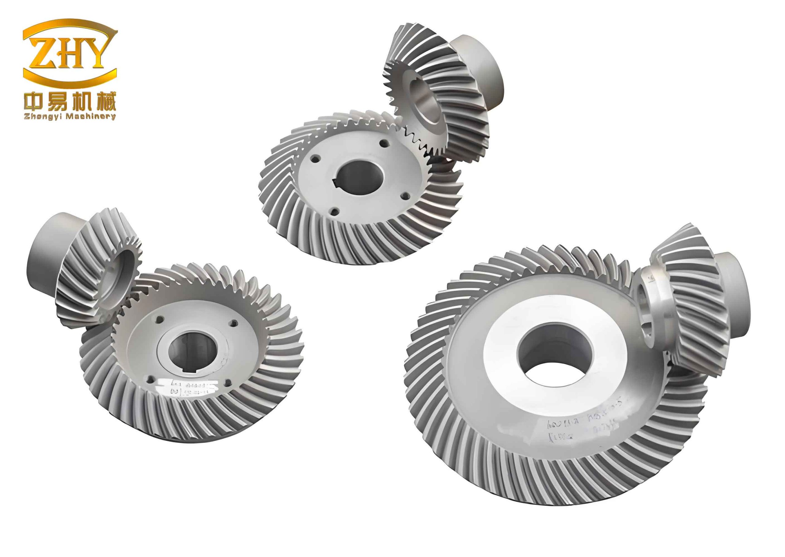
The image above illustrates a typical hyperboloidal gear, highlighting its complex tooth geometry and offset axes. This visual context is essential for understanding the machining challenges. In my work, I have found that accurate calculation of these parameters is not just theoretical but directly impacts manufacturing efficiency and gear performance. For instance, errors in vertical offset or tool position can lead to incorrect tooth contact patterns, causing noise, wear, or even failure in applications like construction machinery. Therefore, I developed a program module to automate these calculations, reducing human error and speeding up the process. The module is based on the formulas derived above and follows a structured workflow.
The program module I designed operates in two main phases: first, the calculation of basic cutting parameters (e.g., cutter data), and second, the computation of machine adjustment settings. It builds upon the geometric design of the hyperboloidal gears, which provides initial parameters such as teeth numbers, offset distance, pitch diameters, and spiral angles. The module’s flowchart, as I implemented it, starts with inputting these geometric parameters, then proceeds to calculate the cutting parameters for both gears, followed by the machine settings. Key steps include selecting cutter specifications (like blade angles and tip radius) based on recommended standards, and iterating if needed for contact pattern optimization. The main interface window allows users to input data easily and view results in tabular form. Below is a table summarizing the core input parameters required for the calculation module, which I commonly use for hyperboloidal gears in engineering contexts:
| Parameter | Symbol | Description | Typical Units |
|---|---|---|---|
| Number of teeth (pinion) | \( Z_1 \) | Teeth count on the small hyperboloidal gear | Dimensionless |
| Number of teeth (gear) | \( Z_2 \) | Teeth count on the large hyperboloidal gear | Dimensionless |
| Offset distance | \( E \) | Axis offset between pinion and gear | mm |
| Pitch diameter (gear) | \( d_{e2} \) | Reference diameter for the large gear | mm |
| Mean cutter radius | \( r_0 \) | Average radius of the cutting tool | mm |
| Face width (gear) | \( b_2 \) | Width of the gear tooth along the axis | mm |
Once the inputs are provided, the module calculates intermediate variables such as cone distances, spiral angles, and limit values. For example, the cone distance \( L_{f2} \) for the large hyperboloidal gear is derived from pitch diameter and root angle. Then, using the formulas for \( L_{c2} \) and \( \varepsilon’_{c2} \), it computes the generating gear parameters. The machine settings \( E_{m2} \), \( X_{b2} \), \( X_2 \), \( S_{d2} \), and \( q_{o2} \) are outputted. Similarly, for the small hyperboloidal gear, the module repeats the process with appropriate substitutions. To handle cutter selection, I incorporated a database of standard cutter specifications, allowing users to choose based on calculated recommendations. This is often presented in a selection window during runtime. For instance, after calculating required blade angles, the program might suggest a cutter with specific profile angles and tip radius from a lookup table. This interactive aspect improves usability, especially for technicians without deep theoretical knowledge.
In practice, I applied this module to a real-world case involving hyperboloidal gears for a YZ10 hydraulic vibratory roller’s drive axle. The input parameters were: \( Z_1 = 5 \), \( Z_2 = 39 \), \( E = 30 \) mm, \( d_{e2} = 318.24 \) mm, \( r_0 = 114.3 \) mm, \( b_2 = 42.5 \) mm. The geometric design module first computed basic dimensions like pitch angles, spiral angles, and root angles. Then, the adjustment module took over. For the large hyperboloidal gear, it calculated \( L_{f2} = 162.45 \) mm, \( \delta_{f2} = 72.5^\circ \), \( \beta_{f2} = 35.2^\circ \). Using the formulas, I derived \( L_{c2} = 150.12 \) mm, \( \varepsilon’_{c2} = 8.3^\circ \), leading to \( E_{m2} = 21.67 \) mm, \( X_{b2} = -5.43 \) mm, \( X_2 = 12.18 \) mm. The radial tool position was \( S_{d2} = 145.89 \) mm, and tool polar angle \( q_{o2} = 42.7^\circ \). For the small hyperboloidal gear, similar computations yielded \( E_{m1} = 18.34 \) mm, \( X_{b1} = -4.12 \) mm, \( S_{d1} = 138.76 \) mm, and \( q_{o1} = 38.5^\circ \). The cutter parameters selected included a dual-sided blade with profile angles of \( 20^\circ \) and \( 25^\circ \), a tip radius of 0.8 mm, and a blade edge radius of 0.2 mm. These results were outputted in a clear format, as shown in the following table summarizing the machining adjustment parameters for both hyperboloidal gears:
| Parameter | Large Hyperboloidal Gear | Small Hyperboloidal Gear |
|---|---|---|
| Vertical gear offset \( E_m \) | 21.67 mm | 18.34 mm |
| Machine center distance \( X_b \) | -5.43 mm | -4.12 mm |
| Gear offset correction \( X \) | 12.18 mm | 10.56 mm |
| Radial tool position \( S_d \) | 145.89 mm | 138.76 mm |
| Tool polar angle \( q_o \) | 42.7° | 38.5° |
| Machine roll ratio \( i_c \) | 1.124 | 1.089 |
The implementation of these calculated settings in the machining workshop proved highly effective. Compared to manual adjustments, the program module reduced setup time by over 50% and minimized trial cuts. Initially, without automation, technicians relied on empirical tables and iterative testing, which often led to multiple machine adjustments and scrap parts. With my module, the calculations are performed instantly, and any changes in cutter parameters (e.g., if a different tool radius is used) can be recalculated swiftly. This is particularly valuable during contact pattern testing: if the initial tooth contact on the hyperboloidal gears is unsatisfactory, the cutter data can be modified, and new adjustment parameters computed within seconds. For the YZ10 roller gears, the first trial showed a contact pattern slightly biased toward the toe; by adjusting the cutter radius from 114.3 mm to 115.0 mm and recomputing, the pattern centered correctly. This agility significantly boosts productivity in manufacturing environments where hyperboloidal gears are produced in batches for construction machinery.
Beyond basic calculations, I enhanced the module to include validation checks and error handling. For instance, it verifies that computed values like \( L_{c2} \) are positive and within machine limits. Additionally, I integrated formulas for stress and durability estimations, though these are optional for users focused solely on machining. The program is written in a high-level language, allowing portability across different computer systems. The user interface features input fields, dropdown menus for standard cutter selections, and graphical outputs for contact pattern simulation. While the core relies on the derived mathematical models, I also incorporated empirical correction factors based on industry practices for hyperboloidal gears. These factors account for material properties and heat treatment effects, which can slightly alter tooth geometry during hardening. For example, a post-heat treatment distortion factor might adjust the calculated machine settings by a small offset, ensuring the final gear meets specifications after all processing stages.
In conclusion, the development of this calculation and program module for hyperboloidal gears has transformed the machining adjustment process. By grounding the software in rigorous mathematical derivations, I ensured accuracy and reliability. The use of tables and formulas within the program aids in transparency, allowing engineers to verify steps if needed. The module’s efficiency is evident in reduced setup times, fewer errors, and improved gear quality. For industries relying on hyperboloidal gears, such as construction machinery, this translates to lower costs and higher performance. Future improvements could include integration with CNC machines for direct setting transmission, or AI-based optimization of cutter parameters to minimize wear. However, the current version already represents a significant advancement. My experience confirms that automating such complex calculations is not just a convenience but a necessity for modern manufacturing of hyperboloidal gears, where precision and speed are paramount.
Throughout this article, I have emphasized the importance of hyperboloidal gears in mechanical systems and the critical role of accurate machining adjustments. The formulas and tables provided serve as a foundation for anyone involved in gear manufacturing. By sharing this methodology, I hope to contribute to broader adoption of computational tools in the field, ultimately enhancing the production of hyperboloidal gears for various engineering applications. The success in real-world cases, like the YZ10 roller, underscores the practicality of this approach. As technology evolves, I anticipate further refinements, but the core principles outlined here will remain essential for mastering the art of hyperboloidal gear machining.