
Hypoid gears are among the most important machine elements in automotive rear-axle drives. They transmit motion between crossed axes by means of hyperboloid tooth surfaces, and they offer a number of advantages over ordinary bevel gears. In particular, the pinion axis can be offset from the gear axis, which makes it possible to lower the vehicle floor, to improve ride comfort, and to obtain a more compact rear-axle assembly. Hypoid gears also have a high contact ratio, a high load-carrying capacity, and relatively smooth meshing behavior. However, these advantages are strongly dependent on the accuracy of the gear geometry and on the precision of the mounting positions. In practice, a set of hypoid gears that has been designed and tested on a rolling test machine can still generate excessive noise and an unfavourable contact pattern when installed in a vehicle because assembly errors and the elastic deformation of supporting structures change the relative position of the gear axes. The purpose of my research was therefore to investigate the contact characteristics of hypoid gears under assembly errors and support deformation, and to provide a theoretical basis for improving gear design and for compensating axis misalignment.
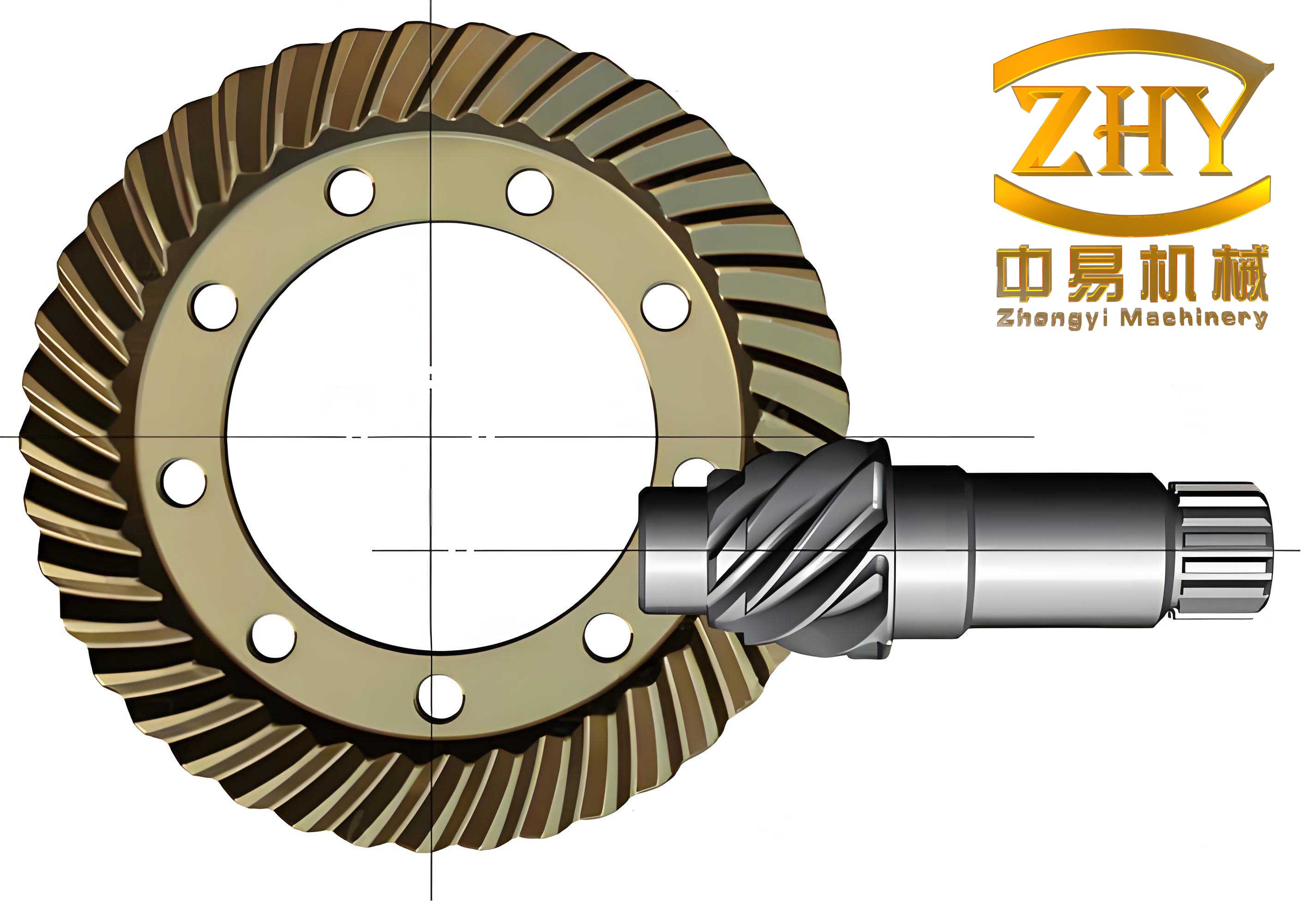
Throughout the work, I focused on face-milled hypoid gears manufactured by the Formate method for the gear and by a generated method for the pinion. My study began with the derivation of the blank geometry and the cutting parameters. Then I generated accurate tooth surfaces and built solid models of the gear and pinion. After that, I performed tooth contact analysis under both ideal and misaligned assembly conditions. I defined a dimensionless sensitivity index for the four basic assembly errors, namely the pinion axial error, the gear axial error, the offset error, and the shaft angle error. Using this index, I optimized the preset parameters used in the local synthesis method and studied how small deviations of the cutting parameters affected the sensitivity. In the final part of the work, I established a complete hypoid gear drive model including the pinion shaft, gear shaft, four tapered roller bearings, and a simplified rear-axle housing. The bearing stiffness matrices were calculated numerically and the bearings were represented by bushings in the finite element model. The finite element analysis provided the tooth contact pressure, the contact regions, and the equivalent axis misalignment of the hypoid gears caused by support deformation.
1. Fundamental Geometry and Cutting Parameters
The accurate generation of the tooth surfaces of hypoid gears is the first step in any theoretical contact analysis. In this section, I describe the calculation of the blank parameters and the cutting parameters for both the gear and the pinion. The gear blank dimensions were calculated according to the standard design procedure for hypoid gears with a double-tapered tooth system. The small gear had 11 teeth and the large gear had 41 teeth, with a pinion offset of 25.4 mm and an outer pitch diameter of 180 mm for the gear. The initial gear face width was chosen as 28 mm, the cutter radius for the gear was 76.2 mm, and the mean spiral angle of the gear was initially set to 50°. Additional parameters such as the pressure angle, the addendum factor, the dedendum factor, and the profile shift coefficients were selected in accordance with common practice for automotive hypoid gears. The most important blank parameters obtained from the iterative calculation are listed in Table 1.
| Parameter | Pinion | Gear |
|---|---|---|
| Number of teeth | 11 | 41 |
| Mean normal module / mm | 3.1758 | |
| Face width / mm | 32.0859 | 28.0000 |
| Mean spiral angle / ° | 49.9931 | 31.8870 |
| Face angle / ° | 22.2802 | 71.6804 |
| Pitch angle / ° | 18.4219 | 70.6804 |
| Root angle / ° | 17.4677 | 66.6804 |
| Mean addendum / mm | 4.1285 | 2.2230 |
| Mean dedendum / mm | 3.0170 | 4.9224 |
| Mean chordal addendum / mm | 4.1735 | 2.2248 |
| Mean chordal tooth thickness / mm | 5.9262 | 3.9050 |
For the gear cutting process, I considered both the Formate method and the generated method. Since the gear pair had a transmission ratio larger than 2.5, the Formate method was the more efficient option and was used in the final gear model. In the Formate method, the gear tooth slots are generated by a face-mill cutter whose axis is fixed in the machine coordinate system while the gear blank is either stationary or rotates only to index the next tooth. The cutter position is determined by the horizontal setting \(H_2\), the vertical setting \(V_2\), the machine root angle \(\gamma_{m2}\), and the axial position of the blank. The following equations describe the basic machine settings for the Formate method:
\[
\gamma_{m2} = \delta_{f2}
\]
\[
V_2 = r_{c0} \cos \beta_{m2}
\]
\[
H_2 = R_{m2}\cos\delta_2 + O_{P2}O_2\cos\gamma_{m2} – r_{c0}\sin\beta_{m2}
\]
In these equations, \(\delta_{f2}\) is the dedendum angle of the gear, \(r_{c0}\) is the cutter radius, \(\beta_{m2}\) is the mean spiral angle, \(R_{m2}\) is the mean cone distance, and \(O_{P2}O_2\) defines the relative position between the pitch apex and the crossing point of the gear axes. The blade pressure angles and the point width of the gear cutter were not simply taken equal to the nominal values. Instead, I treated them as unknowns and solved a nonlinear system of equations that imposed the mean chordal tooth thickness and the mean chordal addendum at the middle of the tooth width. This is a more general approach and it makes the theoretical tooth thickness consistent with the blank data.
For the generated gear cutting process, the blank and the cradle rotate relative to each other according to a ratio \(R_{a2}\), and the tooth surface is formed as the envelope of the family of cutter surfaces. The relative angular displacement satisfies
\[
\theta_2 = R_{a2}\,\varphi_2
\]
where \(\theta_2\) is the rotation of the gear blank and \(\varphi_2\) is the rotation of the cradle. The generated gear cutting parameters include the horizontal and vertical settings, the machine root angle, the horizontal wheel position, the sliding base position, and the roll ratio. The resulting gear cutting parameters for both methods are listed in Table 2 for the particular gear pair used in my study.
| Gear cutting parameter | Formate method | Generated method |
|---|---|---|
| Horizontal cutter setting / mm | 41.2464 | 40.9200 |
| Vertical cutter setting / mm | 64.7088 | 64.7088 |
| Horizontal wheel position / mm | 0 | 0.7572 |
| Vertical wheel position / mm | 0 | 0 |
| Machine root angle / ° | 66.6804 | 66.6804 |
| Sliding base position / mm | 0.6790 | -0.1456 |
| Roll ratio | – | 1.0571 |
| Outside blade pressure angle / ° | 19.2647 | 18.0242 |
| Inside blade pressure angle / ° | 23.5540 | 22.2488 |
| Blade point width / mm | 2.2572 | 2.4721 |
The gear tooth surface is represented in the gear fixed coordinate system by applying a sequence of coordinate transformations to the blade cutting edge. For the Formate method, the position vector of a point on the gear tooth surface is written as
\[
\mathbf r_{2}(s_2,t_2) = \mathbf M_{2,m2}\mathbf M_{m2,c2}\mathbf M_{c2,t2}\,\mathbf r_{t2}(s_2,t_2)
\]
where \(s_2\) and \(t_2\) are the blade length and the cutter rotation parameters, respectively. For the generated method, the cradle rotation \(\varphi_2\) must also be included, and the gear tooth surface is obtained as the envelope of the family of tool surfaces, which leads to the meshing condition
\[
\left(\frac{\partial \mathbf r_2}{\partial s_2} \times \frac{\partial \mathbf r_2}{\partial t_2}\right)\cdot \frac{\partial \mathbf r_2}{\partial \varphi_2} = 0
\]
After solving this equation together with the coordinate equations, the complete gear tooth surface can be generated.
2. Pinion Cutting Parameters by Local Synthesis
The pinion of a hypoid gear pair cannot be cut by the same simple Formate method because the pinion must be conjugated to the gear. The standard approach is to obtain the pinion tooth surface by local synthesis. The goal of local synthesis is to make the pinion and the gear contact at a prescribed point with prescribed transmission error, contact ellipse size, and contact path direction. In my implementation, I fixed the gear tooth surface and computed the pinion cutting parameters that produce the desired contact properties at the mean contact point.
The local synthesis method requires three preset parameters. The first is the maximum transmission error \(\mathit{err}\). The second is the length of the major semi-axis of the contact ellipse \(a\). The third is the direction of the contact path on the gear tooth surface, represented by the angle \(\eta_2\). I used the following ranges during the parametric study:
| Preset parameter | Symbol | Range |
|---|---|---|
| Transmission error | \(\mathit{err}\) | 4.9″ – 30″ |
| Contact ellipse semi-major axis | \(a\) | 2.8 – 7.0 mm |
| Contact path direction | \(\eta_2\) | 0° – 90° |
The pinion tooth surface is generated by a single-side face-mill cutter with a tilting mechanism. The vector equation of the pinion surface can be written in the form
\[
\mathbf r_1(s_1,t_1,\theta_1) = \mathbf M_{1P}\mathbf M_{P6}\mathbf M_{6,m1}\mathbf M_{m1,5}\mathbf M_{5,4}\mathbf M_{4,3}\mathbf M_{3,c1}\mathbf M_{c1,t1}\,\mathbf r_{t1}(s_1,t_1)
\]
where \(s_1\) and \(t_1\) define the position on the cutting edge, and \(\theta_1\) is the rotation of the pinion blank during generating. The unit normal vector of the pinion tooth surface is
\[
\mathbf n_1 = \frac{\partial \mathbf r_1}{\partial s_1} \times \frac{\partial \mathbf r_1}{\partial t_1}
\]
The meshing condition between the cutter and the pinion blank is
\[
\mathbf n_1 \cdot \frac{\partial \mathbf r_1}{\partial \theta_1} = 0
\]
The unknown cutting parameters are the radial setting \(S_{r1}\), the initial cradle angle \(q\), the tilting angle \(i\), the swivel angle \(j\), the vertical wheel position \(E_{m1}\), the horizontal wheel position \(X_{b1}\), the sliding base position \(X_{p1}\), the machine root angle \(\gamma_{m1}\), the roll ratio \(R_{a1}\), the cutter radius \(r_{p1}\), and the blade pressure angle \(\alpha_p\). Together with the surface parameters at the mean point, these unknowns are solved from ten nonlinear equations that express equality of positions, collinearity of normals, equality of principal directions at the contact point, and equality of principal curvatures. In the local synthesis method, the first and second order geometric properties of the gear tooth surface are known, and the corresponding properties of the pinion surface at the mean contact point are determined from the chosen transmission error, contact ellipse, and contact path direction.
In conventional practice, the pinion cutter blades are straight. However, circular blades and parabolic blades have been used to improve the contact behavior and to reduce edge contact. My method is general enough to handle these blade shapes. For a circular arc cutting edge, the blade edge is described by a circular arc of radius \(R\) with a center determined by the pressure angle and the nominal cutter radius. For a parabolic cutting edge, the edge is described by a quadratic function \(x = c s^2\), where \(c\) is the parabolic coefficient. I applied the same local synthesis procedure to these two non-straight blade forms. Tables 4 and 5 list the pinion cutting parameters for the straight, circular, and parabolic blade profiles.
| Pinion cutting parameter | Straight blade (concave) | Circular blade (radius 762 mm) | Parabolic blade (c = 0.0008) |
|---|---|---|---|
| Cutter radius / mm | 67.1104 | 69.6272 | 70.1729 |
| Radial setting / mm | 64.8029 | 64.4800 | 64.3835 |
| Initial cradle angle / ° | 81.8607 | 81.5249 | 81.4432 |
| Tilting angle / ° | 15.8107 | 15.8107 | 15.8107 |
| Swivel angle / ° | 307.6424 | 307.3066 | 307.2249 |
| Horizontal wheel position / mm | 23.9368 | 23.9162 | 23.9119 |
| Vertical wheel position / mm | 23.3653 | 21.4580 | 21.0165 |
| Sliding base position / mm | -7.9521 | -5.6292 | -5.1201 |
| Roll ratio | 3.3152 | 3.3005 | 3.2961 |
The tooth surfaces of hypoid gears are not analytical surfaces that can be represented by simple closed-form expressions. I therefore generated a dense set of points on the working flank and on the transition surface by solving the meshing equations for a large number of discrete surface parameters. For the gear, I sampled 40 points along the blade length and 20 points along the cutter rotation range for the working flank, and 10 by 40 points for the transition surface. For the pinion, the corresponding meshing equation had to be solved using a nonlinear solver for every grid point. The resulting point clouds were fitted by NURBS surfaces using reverse engineering software, and the surfaces were subsequently imported into solid modeling software. The final gear and pinion solid models were obtained by performing a Boolean subtraction between the fitted tooth slot surfaces and the blank geometry, followed by a circular pattern of the tooth slots around the gear and pinion axes.
3. Tooth Contact Analysis
Tooth contact analysis (TCA) is an indispensable tool for the design and optimization of hypoid gears. In my TCA model, I placed the gear and pinion in a fixed reference frame and allowed the pinion to rotate by an angle \(\psi_1\) while the gear rotates by \(\psi_2\). The gear and pinion tooth surfaces are transformed into the fixed frame using the following coordinate transformation matrices:
\[
\mathbf r_1^{(f)}(s_1,t_1,\psi_1) = \mathbf M_{f1}(\psi_1)\mathbf r_1(s_1,t_1)
\]
\[
\mathbf r_2^{(f)}(s_2,t_2,\psi_2) = \mathbf M_{f2}(\psi_2)\mathbf r_2(s_2,t_2)
\]
At every instant of meshing, the two surfaces must satisfy the condition of contact, which implies that the position vectors and the surface normals coincide. This can be written as
\[
\mathbf r_1^{(f)}(s_1,t_1,\psi_1) – \mathbf r_2^{(f)}(s_2,t_2,\psi_2) = \mathbf 0
\]
\[
\mathbf n_1^{(f)} \cdot \frac{\partial \mathbf r_2^{(f)}}{\partial s_2} = 0,\qquad
\mathbf n_1^{(f)} \cdot \frac{\partial \mathbf r_2^{(f)}}{\partial t_2} = 0
\]
Because the pinion tooth surface is an implicit function of \(s_1\), \(t_1\), and \(\theta_1\), the meshing equation of the pinion is added to the system of equations. I used a Newton-type solver in MATLAB to solve the resulting six-by-six nonlinear system for a sequence of pinion rotation angles. The contact point coordinates were then plotted on the gear tooth surface and on the pinion tooth surface to obtain the contact path.
For the theoretical installation, the contact path on the gear convex flank moved from the top/toe region to the root/heel region when the pinion concave flank was the driving side. This behavior is typical for a correctly designed hypoid gear pair and confirmed that the calculated cutting parameters and the solid models were consistent. The transmission error curve was also smooth and had a parabolic shape, which is desirable for low noise and vibration.
4. Assembly Error Sensitivity of Hypoid Gears
In service, the relative position of the pinion and gear axes differs from the theoretical position because of manufacturing tolerances, wear, deflections, and thermal effects. For hypoid gears, four independent assembly errors are usually considered: the pinion axial displacement \(\Delta P\), the gear axial displacement \(\Delta G\), the offset error \(\Delta E\), and the shaft angle error \(\Delta \Sigma\). In my study, I represented the misaligned gear pair by introducing these four errors into the TCA coordinate transformations. I then computed the contact point that corresponds to the theoretical transmission ratio and compared it with the ideal contact point.
To quantify the effect of each assembly error, I defined an error sensitivity index \(\varphi_d\). Let \(d\) be the distance between the ideal contact point and the contact point under a given assembly error, and let \(\alpha\) be the angle between the line joining these two points and the root line of the gear tooth. The normalized sensitivity is defined as
\[
\varphi_d = \frac{d}{m_{mn}\,\sin\alpha}
\]
where \(m_{mn}\) is the mean normal module of the gear pair. This index accounts for both the magnitude and the direction of the shift. I evaluated the sensitivity for assembly errors in the range of -0.1 to 0.1 mm for linear errors and -0.1° to 0.1° for the angular error. The results are summarized in Table 6.
| Assembly error type | Pinion sensitivity range | Gear sensitivity range | Observation |
|---|---|---|---|
| Offset error \(\Delta E\) | 0.12 – 1.15 | 0.10 – 1.12 | Lowest overall sensitivity |
| Gear axis error \(\Delta G\) | 0.25 – 1.60 | 0.20 – 1.55 | Moderate sensitivity |
| Shaft angle error \(\Delta \Sigma\) | 0.30 – 1.44 | 0.20 – 1.80 | Asymmetric positive/negative behavior |
| Pinion axis error \(\Delta P\) | 0.40 – 2.30 | 0.35 – 2.20 | Highest sensitivity among the four errors |
The pinion axial error caused the largest shift of the contact pattern. This result is important because the pinion of an automotive rear axle is usually supported as a cantilever, and its axial position is strongly affected by bearing clearance and housing flexibility. The offset error, on the other hand, had the smallest effect when the error was below 0.05 mm. The shaft angle error produced a different behavior for positive and negative values; positive shaft angle errors were less critical than negative ones. The gear axial error was slightly more critical for the pinion than for the gear.
I also studied how the three preset parameters of local synthesis affect the assembly error sensitivity. The transmission error \(\mathit{err}\) had the strongest influence on the shaft angle sensitivity and the pinion axial sensitivity. Increasing \(\mathit{err}\) from 5″ to 25″ reduced the sensitivity by a factor of about two, but after 20″ the reduction became small. The contact ellipse size \(a\) mainly affected the offset error sensitivity. A larger contact ellipse reduced the offset sensitivity because the contact pattern was naturally wider and could tolerate small positional shifts. The contact path direction \(\eta_2\) affected the gear axial sensitivity and the shaft angle sensitivity in opposite ways. The gear axial sensitivity increased when \(\eta_2\) increased, while the shaft angle sensitivity decreased. The best overall range of \(\eta_2\) was between 45° and 75°, where the four sensitivities were balanced.
Because the preset parameters strongly influence the contact quality of hypoid gears, I formulated an optimization problem with the objective function
\[
\min f(a, \mathit{err}, \eta_2) = c_1\varphi_E + c_2\varphi_G + c_3\varphi_P + c_4\varphi_\Sigma
\]
where \(\varphi_E\), \(\varphi_G\), \(\varphi_P\), and \(\varphi_\Sigma\) are the sensitivity values for the offset, gear axial error, pinion axial error, and shaft angle error, respectively. The weighting coefficients \(c_1\) through \(c_4\) were all set to 0.25. The optimization was performed by discrete search over the feasible ranges. The final optimized preset parameters and the resulting sensitivity reductions are given in Tables 7 and 8.
| Preset parameter | Before optimization | After optimization |
|---|---|---|
| Contact ellipse semi-major axis / mm | 5.04 | 4.48 |
| Transmission error / ″ | 8 | 12 |
| Contact path direction / ° | -65 | -78.3 |
| Sensitivity variable | Before optimization | After optimization | Reduction / % |
|---|---|---|---|
| Offset sensitivity | 1.1182 | 1.0082 | 9.94 |
| Gear axial sensitivity | 1.2820 | 1.0840 | 15.44 |
| Pinion axial sensitivity | 2.3036 | 1.4919 | 35.24 |
| Shaft angle sensitivity | 1.6805 | 0.8111 | 51.73 |
| Weighted objective | 1.5961 | 1.0998 | 31.09 |
After the preset parameters were optimized, I investigated how small deviations in the pinion cutting parameters changed the assembly error sensitivity. The length parameters were varied over \(\pm 0.1\,\text{mm}\), the angle parameters over \(\pm 0.2^\circ\), and the roll ratio over \(\pm 0.002\). The results showed that the cutter radius, the radial setting, and the sliding base position had the largest influence on sensitivity. A negative deviation of the radial setting increased the sensitivity to shaft angle errors. In contrast, a positive deviation of the blade pressure angle reduced the pinion axial sensitivity but increased the gear axial sensitivity. These findings can be used to adjust the pinion cutting process when a particular type of assembly error is expected in the final drive housing.
5. Support Deformation and Loaded Tooth Contact Analysis
The TCA model in the previous section only considered geometric assembly errors, but the actual deformation of the shaft-bearing-housing system also changes the relative position of the gear axes. In this section, I describe the loaded tooth contact analysis of hypoid gears in a complete rear-axle supporting structure.
The finite element model consisted of the pinion shaft, the gear shaft, the gear blank, a simplified differential housing, and a simplified axle housing. The pinion was integral with its shaft, while the large gear was connected to the differential housing by a bolted joint. I did not include the differential gears or the wheel shafts, because their influence on the gear meshing was small compared with that of the main bearings and the housing. The four bearings were tapered roller bearings: two for the pinion shaft and two for the gear shaft. Figure 1 shows the layout of the bearings in the system.
| Bearing designation | Type | Position |
|---|---|---|
| \(b_{11}\) | 30207 | Pinion front bearing |
| \(b_{12}\) | 30206 | Pinion rear bearing |
| \(b_{21}\), \(b_{22}\) | 30209 | Gear differential bearings |
In order to obtain the bearing stiffness matrices, I first calculated the forces acting on the pinion and the gear from the gear meshing force equations. For an input torque \(T_1 = 500\,\text{N·m}\), the tangential, radial, and axial force components on the pinion are:
\[
F_{mt1} = \frac{2000\,T_1}{d_{m1}}
\]
\[
F_{r1} = F_{mt1}\frac{\tan\alpha_D \cos\delta_1 – \tan\beta_{m1}\sin\delta_1}{\cos\beta_{m1}}
\]
\[
F_{a1} = F_{mt1}\frac{\tan\alpha_D \sin\delta_1 + \tan\beta_{m1}\cos\delta_1}{\cos\beta_{m1}}
\]
Similar equations were used for the gear. Then, using the equilibrium of forces and moments for the pinion shaft and the gear shaft, I determined the radial loads of the four bearings. The axial loads of the tapered roller bearings were obtained from the internal axial force balance. The bearing loads at the nominal torque are listed in Table 10.
| Bearing | \(F_x\) / N | \(F_y\) / N | \(F_z\) / N |
|---|---|---|---|
| \(b_{11}\) | 2.3159×10⁴ | -5.2536×10³ | 2.7004×10⁴ |
| \(b_{12}\) | 4.9734×10³ | 8.1146×10³ | 2.9742×10³ |
| \(b_{21}\) | 1.3199×10⁴ | 1.4008×10⁴ | 8.5372×10³ |
| \(b_{22}\) | 1.0844×10⁴ | 3.7698×10³ | 3.8269×10³ |
The stiffness matrix of a tapered roller bearing can be derived from the load-displacement relationship of the rolling elements. Let \(\delta_{rj}\) and \(\delta_{zj}\) be the radial and axial displacements of the \(j\)-th rolling element. The equilibrium equations for the bearing forces are
\[
\sum_{j=1}^{N} K_n \left(\delta_{rj}\cos\alpha + \delta_{zj}\sin\alpha\right)^{10/9} \cos\alpha \cos\varphi_j = F_x
\]
\[
\sum_{j=1}^{N} K_n \left(\delta_{rj}\cos\alpha + \delta_{zj}\sin\alpha\right)^{10/9} \cos\alpha \sin\varphi_j = F_y
\]
\[
\sum_{j=1}^{N} K_n \left(\delta_{rj}\cos\alpha + \delta_{zj}\sin\alpha\right)^{10/9} \sin\alpha = F_z
\]
where \(\alpha\) is the contact angle, \(\varphi_j\) is the angular position of the rolling element, and \(K_n\) is the load-deflection coefficient. After solving the equilibrium equations by the Newton-Raphson method, the \(3 \times 3\) bearing stiffness matrix is obtained as the Jacobian matrix of the load vector with respect to the displacement vector:
\[
\mathbf K_b = \frac{\partial (F_x, F_y, F_z)}{\partial (\delta_x, \delta_y, \delta_z)}
\]
The calculated stiffness matrices at the nominal load are given below for the four bearings.
For the pinion front bearing \(b_{11}\),
\[
\mathbf K_{b11} =
\begin{bmatrix}
1.8694\times10^6 & 1.6886\times10^4 & 4.1380\times10^5 \\
& 1.8765\times10^6 & -4.6935\times10^4 \\
& & 2.3044\times10^6
\end{bmatrix}
\ \text{N/mm}
\]
For the pinion rear bearing \(b_{12}\),
\[
\mathbf K_{b12} =
\begin{bmatrix}
7.7341\times10^5 & 6.2335\times10^3 & 2.2811\times10^5 \\
& 7.6643\times10^5 & 2.1090\times10^4 \\
& & 9.3321\times10^5
\end{bmatrix}
\ \text{N/mm}
\]
For the gear bearing \(b_{21}\),
\[
\mathbf K_{b21} =
\begin{bmatrix}
1.4405\times10^6 & -2.4586\times10^4 & 3.2194\times10^5 \\
& 1.4245\times10^6 & 1.6782\times10^5 \\
& & 2.0887\times10^6
\end{bmatrix}
\ \text{N/mm}
\]
For the gear bearing \(b_{22}\),
\[
\mathbf K_{b22} =
\begin{bmatrix}
9.0533\times10^5 & 7.0967\times10^4 & 5.9503\times10^5 \\
& 7.1699\times10^5 & 9.8015\times10^4 \\
& & 1.1827\times10^6
\end{bmatrix}
\ \text{N/mm}
\]
In the finite element model, each bearing was replaced by a bushing connection with the corresponding stiffness matrix. The bushing elements connected the shaft nodes to the housing nodes. The contact between the pinion and the gear was modeled as frictional contact with a friction coefficient of 0.1. The pinion shaft was driven by a torque of 500 N·m, and the outer surfaces of the axle housing were fixed. The material properties used in the analysis are listed in Table 11.
| Component | Material | Elastic modulus / GPa | Poisson ratio | Density / kg·m⁻³ |
|---|---|---|---|---|
| Pinion and gear | 20CrMnTi | 207 | 0.25 | 7800 |
| Axle housing | KT350-10 | 155 | 0.23 | 7200 |
The mesh was refined only in the expected contact zones of the four pairs of teeth that could be in simultaneous engagement. A mesh size of 0.5 mm was used in the contact zone, while the rest of the model was meshed with a larger element size. The enhanced Lagrange formulation was used in order to reduce penetration and to improve convergence.
6. Results of Loaded Contact Analysis
I first evaluated the contact state for different angular positions of the gear pair. The number of tooth pairs in contact changed as the gears rotated. At the mean contact position, three pairs of teeth participated in the load sharing, but the load distribution was not uniform. The highest contact pressure occurred when the contact was near the edge of the tooth, where local stress concentrations were observed. This demonstrates that edge contact is a serious risk in hypoid gears, especially when the supporting system deforms under load.
Next, I applied different torque levels at the same angular position. At \(T = 5\,\text{N·m}\), only one tooth pair was in contact and the contact area was small. As the torque increased, the elastic deflection increased and the contact area expanded. At \(T = 150\,\text{N·m}\), a second tooth pair began to share the load, but an edge contact appeared at one side of the gear tooth. At \(T = 500\,\text{N·m}\), three or four tooth pairs were in contact and the maximum contact pressure increased with the torque. The contact pressures at several torque levels are summarized in Table 12.
| Torque / N·m | Number of contacting pairs | Maximum contact pressure / MPa | Edge contact? |
|---|---|---|---|
| 5 | 1 | 210 | No |
| 50 | 2 | 1120 | No |
| 150 | 2 | 1760 | Yes |
| 350 | 3 | 2150 | Yes |
| 500 | 4 | 2327 | Yes |
The support deformation caused an equivalent displacement of the gear axes. To compute the equivalent misalignment, I monitored the positions of four points on the pinion and gear axes. Let \(O_{11}\) and \(O_{12}\) be two points on the undeformed pinion axis, and \(O_{21}\) and \(O_{22}\) be two points on the undeformed gear axis. After deformation, these points moved to new positions. The unit vectors along the deformed axes are
\[
\mathbf e_1 = \frac{\mathbf O’_{12} – \mathbf O’_{11}}{|\mathbf O’_{12} – \mathbf O’_{11}|}
\]
\[
\mathbf e_2 = \frac{\mathbf O’_{22} – \mathbf O’_{21}}{|\mathbf O’_{22} – \mathbf O’_{21}|}
\]
The vector along the common perpendicular of the deformed axes is
\[
\mathbf n = \mathbf e_1 \times \mathbf e_2
\]
From these quantities, the equivalent pinion axial error, gear axial error, offset error, and shaft angle error were derived. The results are shown in Table 13 for three modeling levels: shaft only, shaft with bearings, and the complete shaft-bearing-housing system.
| Equivalent misalignment | Shaft only | Shaft + bearings | Shaft + bearings + housing |
|---|---|---|---|
| \(\Delta P\) / μm | 72.2 | 82.6 | 104.0 |
| \(\Delta G\) / μm | 141.2 | 93.1 | 129.5 |
| \(\Delta E\) / μm | -167.2 | -156.9 | -238.7 |
| \(\Delta \Sigma\) / ° | 0.0673 | 0.0469 | 0.0589 |
The results indicate that the housing deformation had a significant contribution to the equivalent offset error and the pinion axial error. The offset error was the largest in the complete system, reaching about -239 μm at 500 N·m. This is larger than the typical manufacturing tolerance and cannot be neglected. The gear axial error was reduced when the bearings were included, because the bearings allowed some axial flexibility that partly compensated the shaft bending. The shaft angle error was small but still large enough to alter the contact path.
Finally, I used the equivalent misalignment values as input to the TCA program in order to predict the actual contact pattern under load. The contact path on both the pinion and the gear shifted toward the toe of the tooth compared with the theoretical contact path. This shift was mainly caused by the combination of the offset error and the pinion axial error. The amount of the shift was about one-third of the tooth width at the nominal torque. This finding confirms that support deformation must be considered during the design stage of hypoid gears, and compensation methods such as modified pinion tooth surfaces or adjusted mounting distances should be used to keep the contact pattern within the central part of the tooth.
7. Conclusions
In this thesis, I systematically investigated the contact characteristics of hypoid gears under assembly errors and support deformation. The main conclusions are as follows.
First, I derived the blank geometry and the cutting parameters for face-milled hypoid gears using the Formate method for the large gear and the generated method for the small gear. The local synthesis method was extended to straight, circular, and parabolic blade profiles, and the corresponding pinion cutting parameters were obtained by solving nonlinear equations. The resulting tooth surfaces were fitted from point clouds and used to build solid models of the gear and the pinion, which provided a reliable basis for contact analysis and finite element analysis.
Second, the tooth contact analysis under ideal installation showed that the contact path had the expected direction and smooth transmission error. The assembly error sensitivity analysis revealed that the pinion axial error was the most critical assembly error for the gear pair, while the offset error was the least critical. The sensitivity could be reduced significantly by optimizing the preset transmission error, contact ellipse size, and contact path direction. The optimized design reduced the weighted sensitivity by about 31%, and the shaft angle sensitivity was reduced by more than 50%. The analysis of cutting parameter deviations also showed that the radial setting and the blade pressure angle had important influences on the sensitivity of hypoid gears.
Third, the loaded tooth contact analysis of the complete hypoid gear drive, including shafts, bearings, and housing, showed that support deformation causes a large equivalent axis misalignment. The offset error was as high as -239 μm at 500 N·m, which is far beyond typical assembly tolerances. The contact pattern shifted toward the toe of the gear tooth, and edge contact appeared when the torque reached about 150 N·m. These results emphasize the importance of considering the stiffness of the supporting system in the design process of hypoid gears. The equivalent misalignment calculated by the finite element method can be used to modify the pinion tooth surface or to adjust the shim thickness in the final drive, thereby improving the meshing quality and the service life of the hypoid gears.