
The analysis of transmission error (TE) is paramount for evaluating the dynamic performance, noise, and vibration characteristics of gear transmissions. Hyperboloid gears, known for their high load capacity and smooth power transfer in non-intersecting axes applications, are particularly sensitive to geometric imperfections. Traditional simulation studies predominantly rely on theoretically perfect tooth surfaces designed via gear generation principles. However, a significant evaluation gap exists when these simulation results, derived from ideal geometry, are compared against physical testing performed on actual manufactured gears, which inherently contain surface deviations introduced during production (cutting, heat treatment, grinding). This inconsistency in the evaluation baseline undermines the predictive accuracy of simulation models for real-world performance. Therefore, this study aims to bridge this gap by constructing and analyzing a simulation model based on the real tooth flank geometry of manufactured hyperboloid gears, thereby providing a more accurate assessment of transmission error and its sensitivity to assembly misalignments.
This research constructs a three-dimensional digital model of a hyperboloid gear pair by applying Non-Uniform Rational B-Spline (NURBS) surface fitting to coordinate data measured directly from production gears. The transmission error of this real-flank model is analyzed using nonlinear finite element methods and compared against that of a theoretically perfect flank model. Subsequently, the influence of key installation errors—axial misalignment of the pinion (ΔH), axial misalignment of the gear (ΔE), offset distance error (ΔV), and shaft angle error (ΔΣ)—on the transmission error is systematically investigated. The sensitivity of TE fluctuation amplitude to each error is quantified. Finally, the validity of the real tooth surface simulation model is corroborated through physical roll testing on a gear checking machine.
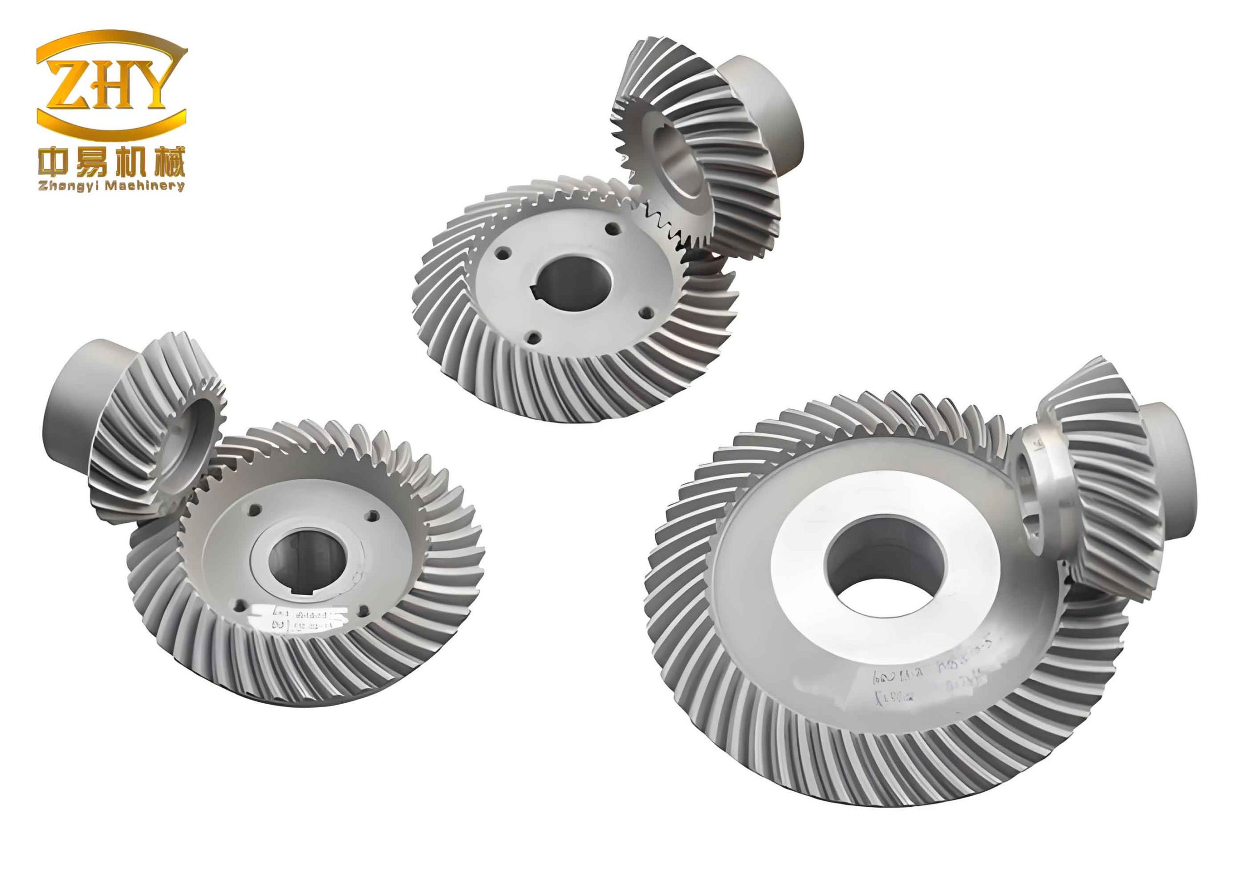
Acquisition and Mathematical Reconstruction of Real Tooth Flanks
The first critical step is to capture the actual geometry of the manufactured hyperboloid gear teeth. Due to the complex spatial curvature of hyperboloid gear flanks, a high-precision coordinate measuring machine (CMM), specifically designed for gear inspection, is employed. For efficient yet comprehensive measurement, a grid of points is defined on the tooth surface: typically, 9 points along the profile (face width) direction and 5 points along the lengthwise (tooth height) direction, resulting in 45 discrete points per flank for both the convex and concave sides of the pinion and gear. An excerpt of the measured 3D coordinates (in a machine coordinate system) for the pinion convex flank is presented below.
| Point ID | X (mm) | Y (mm) | Z (mm) |
|---|---|---|---|
| P11 | 20.0185 | 0.6118 | -35.0599 |
| P12 | 20.5333 | 0.4281 | -34.7572 |
| P13 | 21.0469 | 0.1968 | -34.4543 |
| … | … | … | … |
| P95 | 27.8953 | -1.0300 | -41.5420 |
To reconstruct a continuous geometric model from these discrete points, the NURBS surface fitting technique is utilized, which is highly effective in reverse engineering for complex free-form surfaces. A NURBS surface offers great flexibility in representing sculptured surfaces. A NURBS curve of degree p is defined by:
$$C(u) = \frac{\sum_{i=0}^{n} N_{i,p}(u) w_i P_i}{\sum_{i=0}^{n} N_{i,p}(u) w_i}$$
where \(P_i\) are the control points, \(w_i\) are the corresponding weights, and \(N_{i,p}(u)\) are the B-spline basis functions of degree p. This rational form allows exact representation of conic sections and free-form curves.
Extending to a surface, a NURBS surface of degree p in the u-direction and degree q in the v-direction is defined by:
$$S(u,v) = \frac{\sum_{i=0}^{m} \sum_{j=0}^{n} N_{i,p}(u) N_{j,q}(v) w_{i,j} P_{i,j}}{\sum_{i=0}^{m} \sum_{j=0}^{n} N_{i,p}(u) N_{j,q}(v) w_{i,j}}$$
where \(P_{i,j}\) forms a bidirectional control net, \(w_{i,j}\) are the weights, and \(N_{i,p}(u)\) and \(N_{j,q}(v)\) are the B-spline basis functions.
In this study, the measured 3D coordinates serve as data points for surface interpolation. A cubic (degree 3) NURBS surface is constructed. By solving for the control points and knot vectors that best fit the measured data points, a smooth mathematical representation of the real tooth flank is obtained. This NURBS surface data is then imported into CAD software (e.g., CATIA) to generate a solid 3D model of the hyperboloid gear pair, preserving the actual manufacturing deviations. This model forms the basis for all subsequent high-fidelity simulations, distinguishing it from models based on purely theoretical flank equations.
Fundamentals of Installation Error and Transmission Error in Hyperboloid Gears
Definition of Installation Errors
The operational performance of a hyperboloid gear pair is highly sensitive to its precise alignment within the housing. Deviations from the nominal assembly position are termed installation errors. For a hypoid or hyperboloid gear set, the four primary errors are defined with respect to the nominal configuration and signed convention as follows:
- Pinion Axial Position Error (ΔH): Displacement of the pinion along its own axis. Positive (+) denotes movement bringing the pinion closer to the gear, while negative (-) denotes movement away.
- Gear Axial Position Error (ΔE): Displacement of the gear along its own axis. Positive (+) denotes movement bringing the gear closer to the pinion.
- Offset Distance Error (ΔV): Vertical displacement of the pinion axis relative to the gear axis. Positive (+) denotes the pinion axis moving downward, increasing the nominal offset.
- Shaft Angle Error (ΔΣ): Angular deviation from the nominal angle between the pinion and gear shafts. Positive (+) denotes an increase in the nominal shaft angle.
These errors, often within tight tolerances (e.g., ±0.06 mm, ±0.06°), critically influence the contact pattern, load distribution, and ultimately, the transmission error of the hyperboloid gear pair.
Definition and Significance of Transmission Error
Transmission Error (TE) is a fundamental metric for assessing gear meshing quality. It is defined as the deviation of the actual angular position of the driven gear from its theoretical position for a given angular position of the driving gear, assuming perfectly rigid and conjugate gears. Mathematically, for a pair with pinion as the driver:
$$TE(\phi_1) = \left( \phi_2 – \phi_2^{(0)} \right) – \frac{N_1}{N_2} \left( \phi_1 – \phi_1^{(0)} \right)$$
where:
- \(\phi_1, \phi_2\) are the actual rotation angles of the pinion and gear, respectively.
- \(\phi_1^{(0)}, \phi_2^{(0)}\) are the initial reference rotation angles.
- \(N_1, N_2\) are the number of teeth on the pinion and gear.
TE is typically expressed in micro-radians (μrad) or arc-seconds. A perfectly conjugate gear pair would have zero TE. In reality, TE exists due to elastic deformations, manufacturing errors, and design modifications like flank crowning. The mean value of TE is often related to the average mesh stiffness and nominal load. The fluctuation amplitude (peak-to-peak value) of TE over a mesh cycle is of paramount importance as it is a primary excitation source for gear whine and vibration. Minimizing and controlling the amplitude and shape of the TE curve are key objectives in quiet gear design. Therefore, analyzing how real flank errors and installation errors affect TE is crucial for optimizing the NVH (Noise, Vibration, and Harshness) performance of hyperboloid gear drives.
Development of a High-Fidelity Finite Element Model for Hyperboloid Gear Analysis
To accurately simulate the nonlinear contact behavior and calculate the transmission error under load, a detailed finite element model is developed. The process involves geometry preparation, meshing, material definition, and setting up complex contact conditions.
Geometry and Meshing Strategy
The 3D CAD models of the pinion and gear, constructed from the NURBS-based real flanks, are imported into a pre-processing software like HyperMesh. A strategic meshing approach is adopted to balance computational accuracy and efficiency. The regions away from the contact zone are meshed with relatively coarse tetrahedral or hexahedral elements. The critical tooth flank surfaces and the fillet regions, where high stress concentrations occur, are discretized with a much finer mesh of first-order or second-order tetrahedral elements (C3D4 or C3D10 in Abaqus). A typical high-quality mesh for a hyperboloid gear pair is characterized by several hundred thousand to millions of elements, ensuring that the contact pressure and deformation are captured with sufficient fidelity. The final assembled FE mesh for the hyperboloid gear pair is shown below (conceptually).
Material Properties, Loads, and Boundary Conditions
The gear material is commonly case-hardened steel, such as 20CrMnTi. The material properties assigned in the linear elastic model are:
| Property | Value | Unit |
|---|---|---|
| Young’s Modulus (E) | 212,000 | MPa |
| Poisson’s Ratio (ν) | 0.3 | – |
| Density (ρ) | 7.8e-9 | Tonnes/mm³ |
To apply loads and constraints, a reference point (RP) is created at the theoretical center of each gear’s bore. This RP is kinematically coupled to all the nodes on the inner surface of the gear’s bore using a rigid body or distributing coupling constraint. This allows loads and boundary conditions to be applied conveniently at the RP.
The analysis is conducted in multiple steps to simulate realistic engagement:
- Initial Contact Step: A very small rotational displacement is applied to the pinion’s RP to eliminate any initial gap or penetration and establish stable contact between the gear teeth.
- Load Application Step: A constant braking torque is applied to the gear’s RP to simulate the resistive load from the driveline.
- Meshing Motion Step: A finite rotation is applied to the pinion’s RP, driving it through several tooth engagement cycles. The resulting reaction torque and the rotational angles of both RPs are recorded.
Boundary conditions restrain all translational degrees of freedom (DOFs) at both the pinion and gear RPs, allowing only rotation about their respective axes.
Contact Definition
The interaction between the pinion and gear tooth flanks is the most critical part of the model. A surface-to-surface contact formulation is used. The finer-meshed, potentially more convex surface (often the pinion convex side) is typically chosen as the slave surface. The penalty contact method with a finite sliding formulation is employed. A Coulomb friction model with a coefficient of 0.1 is often used to account for tangential forces. The contact property controls are set for a dynamic, explicit analysis which is suitable for complex contact conditions and quasi-static loading when properly mass-scaled.
| Setting | Description |
|---|---|
| Contact Type | Surface-to-Surface (Explicit) |
| Master Surface | Gear Tooth Flank (selected face) |
| Slave Surface | Pinion Tooth Flank (selected face) |
| Mechanical Constraint | Penalty Friction, Friction Coeff. = 0.1 |
| Sliding Formulation | Finite Sliding |
Simulation Results: Influence of Real Flanks and Installation Errors
Comparison: Real Flank vs. Theoretical Flank Hyperboloid Gear
Two finite element models are analyzed under identical nominal alignment and load conditions: one with the real (NURBS-fitted) tooth flanks and another with perfectly conjugate theoretical flanks. The calculated transmission error curves over one complete mesh cycle are extracted and compared.
The TE curve from the theoretical flank model exhibits a characteristic parabolic shape, which is often intentionally designed via flank modifications to reduce sensitivity to errors. Its mean value is close to zero, and the fluctuation is smooth with a relatively small amplitude.
In stark contrast, the TE curve from the real flank hyperboloid gear model shows significant differences:
- Shift in Mean Value: The entire TE curve is offset by a constant value (e.g., ~2.5e-3 rad). This static offset is a direct consequence of the systematic deviations present on the manufactured gear flanks, effectively altering the nominal kinematic relationship.
- Increased Fluctuation Amplitude: The peak-to-peak value of the TE fluctuation is substantially larger for the real flank model.
- Distorted Curve Shape: While the overall parabolic trend may remain, the curve is no longer smooth. It exhibits a “saw-tooth” or waviness pattern superimposed on the main parabolic shape. This high-frequency content directly corresponds to the localized geometric errors measured on the tooth surface (lead deviation, profile deviation, etc.). These deviations disrupt the ideal line of contact and cause abrupt changes in the effective gear ratio during meshing.
This comparison conclusively verifies that manufacturing-induced flank errors on a hyperboloid gear not only shift the operational reference point but also significantly amplify the dynamic excitation source (TE fluctuation), which would lead to increased vibration and noise in a real transmission system.
Sensitivity Analysis of Transmission Error to Installation Errors
Using the validated real-flank hyperboloid gear model, a series of simulations are conducted to isolate the effect of each installation error. The principle of a controlled variable is applied: for each simulation run, only one error parameter is varied within its practical tolerance range (±0.06 mm or ±0.06°), while the others are kept at their nominal zero value.
| Installation Error | Symbol | Simulation Range |
|---|---|---|
| Offset Distance Error | ΔV | -0.06 mm to +0.06 mm |
| Pinion Axial Position Error | ΔH | -0.06 mm to +0.06 mm |
| Gear Axial Position Error | ΔE | -0.06 mm to +0.06 mm |
| Shaft Angle Error | ΔΣ | -0.06° to +0.06° |
The key observations from the TE results are summarized below:
1. Offset Distance Error (ΔV):
- Mean TE Shift: The entire TE curve shifts in the positive direction as ΔV increases positively.
- Fluctuation Amplitude: The change in TE amplitude (peak-to-peak) is relatively moderate compared to other errors. The sensitivity is asymmetric: TE amplitude is more sensitive to positive ΔV changes than to negative ones.
- Physical Reason: A change in ΔV primarily shifts the contact path along the lengthwise direction of the tooth. Positive ΔV moves the contact towards the toe/heel, potentially engaging areas with different flank error topography, hence the asymmetric effect.
2. Pinion Axial Position Error (ΔH):
- Mean TE Shift: The entire TE curve shifts in the negative direction as ΔH increases positively. This is opposite to the trend observed for ΔV.
- Fluctuation Amplitude: This error has a very pronounced effect on TE amplitude. Both positive and negative ΔH cause a significant increase in amplitude. Interestingly, a small positive ΔH might result in a slightly smoother TE curve than a negative ΔH, suggesting a partial compensation of the inherent flank errors in that specific direction.
- Physical Reason: ΔH changes the working pressure angle and effectively shifts the contact pattern across the tooth profile (from root to tip). This greatly alters the load distribution and engages different portions of the flank errors, leading to high sensitivity.
3. Gear Axial Position Error (ΔE):
- Mean TE Shift: Similar to ΔH, the TE curve shifts negatively with positive ΔE.
- Fluctuation Amplitude: Among all errors, ΔE has the least influence on the TE fluctuation amplitude. The amplitude remains almost constant across the simulated range.
- Physical Reason: ΔE primarily affects the backlash or clearance between the gears. While it changes the mean mesh position (causing the mean TE shift), it does not drastically alter the fundamental path of contact or the engaged flank geometry relative to each other, hence the low impact on dynamic fluctuation.
4. Shaft Angle Error (ΔΣ):
- Mean TE Shift: The TE curve shifts positively with a positive increase in ΔΣ.
- Fluctuation Amplitude: This is the most sensitive parameter. Any deviation of ΔΣ from nominal, in either direction, causes a dramatic and rapid increase in TE amplitude. A small negative ΔΣ might slightly smooth the curve, but the amplitude still increases considerably.
- Physical Reason: The shaft angle is fundamental to the hyperboloid gear geometry. An error here misaligns the entire kinematic relationship between the flanks, causing severe mismatch and edge loading. It disrupts the conjugate action more fundamentally than axial shifts, leading to the highest sensitivity.
Quantitative Sensitivity Ranking
The peak-to-peak TE amplitude for each error case is plotted against the error magnitude. The slope of these curves at the nominal point (zero error) indicates the sensitivity. Based on the simulation data, the installation errors can be ranked in order of their sensitivity concerning the excitation of TE fluctuations (from highest to lowest):
| Rank | Installation Error | Relative Sensitivity | Key Observation |
|---|---|---|---|
| 1 | Shaft Angle Error (ΔΣ) | Highest | Extreme sensitivity in both directions. |
| 2 | Pinion Axial Error (ΔH) | Very High | High sensitivity, negative error often worse. |
| 3 | Offset Distance Error (ΔV) | Moderate/Asymmetric | More sensitive to positive error. |
| 4 | Gear Axial Error (ΔE) | Lowest | Negligible effect on fluctuation amplitude. |
The relationship can be conceptually expressed as a sensitivity function:
$$ \text{TE}_{\text{amplitude}} \approx f(\Delta\Sigma, \DeltaH, \DeltaV, \DeltaE) $$
where
$$ \left| \frac{\partial f}{\partial \Delta\Sigma} \right| \approx \left| \frac{\partial f}{\partial \DeltaH} \right| > \left| \frac{\partial f}{\partial \DeltaV} \right| > \left| \frac{\partial f}{\partial \DeltaE} \right| \approx 0 $$
Experimental Validation via Gear Roll Testing
To validate the findings from the real-flank finite element model, physical roll tests are conducted on a dedicated gear rolling tester (e.g., a Gleason 600HTT machine). This machine allows precise adjustment of the installation parameters (ΔV, ΔH, ΔE, ΔΣ) and measures the kinematic transmission error under light load.
Experimental Setup and Procedure
The same hyperboloid gear pair used for coordinate measurement is mounted on the tester. The machine’s slides and rotary tables are adjusted to first achieve the “standard” or nominal installation position (all errors set to zero according to the machine’s coordinate system). The pinion is driven at a constant speed (e.g., 500 rpm) under a light braking torque on the gear. The phase difference between the input and output shafts, which is directly proportional to the Transmission Error, is measured with high-resolution encoders and recorded.
Subsequently, controlled deviations are introduced one at a time: ΔV = ±0.04 mm, ΔH = ±0.04 mm, ΔΣ = ±0.06° (approx. ±4 arc-minutes). For each error setting, the roll test is repeated, and the peak-to-peak TE amplitude is recorded.
Comparison of Results: Simulation vs. Experiment
The measured TE amplitudes from the roll tests are compared with the amplitudes predicted by both the theoretical-flank and real-flank FE models. The results for the nominal and various error conditions are consolidated below.
| Condition | Peak-to-Peak Transmission Error Amplitude (μrad) | ||
|---|---|---|---|
| Theoretical Flank FE Model | Real Flank FE Model | Roll Test Experiment | |
| Nominal (All errors=0) | 3.68 | 6.42 | 6.63 |
| ΔV = +0.04 mm | 8.36 | 10.95 | 11.42 |
| ΔV = -0.04 mm | 10.68 | 13.32 | 12.69 |
| ΔH = +0.04 mm | 12.47 | 16.48 | 17.24 |
| ΔH = -0.04 mm | 19.82 | 21.26 | 20.86 |
| ΔΣ = +4′ | 5.68 | 6.84 | 6.80 |
| ΔΣ = -4′ | 4.83 | 6.72 | 6.74 |
Key Observations from Validation:
- The TE amplitude predicted by the real-flank FE model is consistently and significantly closer to the experimentally measured values than the theoretical-flank model for all conditions (nominal and with errors).
- The absolute values and, more importantly, the trends (relative changes due to ΔV, ΔH, ΔΣ) predicted by the real-flank model match the experimental data very well. For instance, both model and experiment show that ΔH has a larger impact than ΔV, and ΔΣ has a severe impact even for small deviations.
- The slight discrepancies between the real-flank simulation and experiment can be attributed to factors not fully captured in the simulation, such as micro-geometry from final finishing, system dynamics of the test rig, and measurement noise.
This strong correlation validates the fundamental premise of this work: using a simulation model based on the real manufactured tooth flank geometry of the hyperboloid gear provides a vastly more accurate and reliable prediction of its functional performance (TE) and its sensitivity to assembly variations, compared to models based on ideal theory alone.
Conclusions and Implications
This comprehensive study on the transmission error of hyperboloid gears based on real tooth surface data leads to the following major conclusions:
- Significance of Real Flank Geometry: Manufacturing-induced deviations on hyperboloid gear tooth flanks have a substantial and quantifiable impact on transmission error. They cause a static shift in the mean TE and, more critically, increase the amplitude and distort the shape of the TE fluctuation curve. Ignoring these real flank errors in simulation leads to an overly optimistic prediction of dynamic performance (noise and vibration).
- Validation of the NURBS-based Modeling Approach: The methodology of reconstructing gear flanks from CMM data using NURBS surfaces and incorporating them into a nonlinear finite element model is validated as a high-fidelity digital twin approach. Its predictions for TE amplitude under various misalignment conditions show excellent agreement with physical roll tests.
- Installation Error Sensitivity: The sensitivity of TE fluctuation amplitude to the four primary installation errors for a hyperboloid gear pair is definitively ranked as: Shaft Angle Error (ΔΣ) ≈ Pinion Axial Error (ΔH) > Offset Error (ΔV) > Gear Axial Error (ΔE). Errors ΔΣ and ΔH are the most critical and must be controlled with the tightest tolerances during the assembly of a hyperboloid gear drive to minimize NVH excitation.
- Error Compensation Effect: It was observed that certain directions of error (e.g., a small positive ΔH or a small negative ΔΣ) could partially smooth the TE curve from the real-flank gear, suggesting a compensatory effect against the specific pattern of manufacturing errors present. This insight could be leveraged in selective assembly or active alignment strategies.
- Practical Guidance: For gearbox designers and assembly engineers working with hyperboloid gears, this research underscores that:
- Simulation-based NVH analysis should strive to incorporate real flank data or statistical representations of manufacturing errors.
- Assembly process design and tolerance allocation should focus intensely on controlling the shaft angle and the pinion’s axial position, as these are the primary levers affecting gear noise.
- Roll testing with controlled misalignments remains an essential tool for final validation and can be effectively guided by the predictions of a real-flank simulation model.
In summary, by bridging the gap between ideal simulation and real manufactured components, this study provides a more robust framework for analyzing and optimizing the transmission error of hyperboloid gears. This contributes directly to the development of quieter, more reliable, and higher-performance gear drives for automotive and industrial applications.