
The increasing deployment of industrial robots has intensified the demand for reliable health monitoring and predictive maintenance. Core to many robotic joints is the rotary vector reducer, a precision gear transmission system prized for its high torque capacity, compact size, and high reduction ratio. Effective fault diagnosis of these reducers is paramount for ensuring robotic system reliability. However, a significant challenge arises from the noisy vibration signals acquired during their operation, especially under the reciprocating motion typical of robotic arms. This reciprocating motion, as opposed to steady-state rotation, often induces non-stationary signal characteristics and makes the collected data highly susceptible to environmental and cross-equipment interference. Therefore, effective denoising of the vibration signals from a rotary vector reducer is a critical preprocessing step for any subsequent diagnostic procedure.
Traditional denoising methods, such as spectral subtraction, wavelet transform, empirical mode decomposition (EMD), and singular value decomposition (SVD), have been applied with some success. For instance, wavelet theory has been used to eliminate noise from rotary vector reducer vibration signals, and EMD-based methods have been employed to extract accurate motion parameters. However, these methods often face limitations, including a heavy reliance on expert knowledge for parameter selection (e.g., wavelet basis, threshold levels, decomposition modes) and difficulty in handling the large, complex datasets now commonly generated. Their performance can be suboptimal when dealing with the specific noise profiles and non-linearities present in signals from reciprocating machinery.
With the advancement of artificial intelligence and big data, deep learning (DL) offers a promising alternative. Unlike traditional algorithms, DL models, particularly Convolutional Neural Networks (CNNs), provide an end-to-end learning framework capable of adaptively learning and extracting relevant features from raw data without extensive manual feature engineering. Models like Fully Convolutional Networks (FCNs) and variations of WaveNet have demonstrated superior denoising capabilities for audio and vibration signals compared to classical filters like the Wiener filter. More recently, Generative Adversarial Networks (GANs) have emerged as a powerful paradigm for learning data distributions and have been successfully adapted for denoising tasks. Yet, most deep learning-based denoising research has focused on components with stable rotational speeds, such as bearings. The application of intelligent denoising models specifically tailored for the vibration signals of a rotary vector reducer operating under reciprocating motion remains underexplored.
To address this gap, this work proposes a novel denoising method based on a Convolutional Auto-encoder Generative Adversarial Network (CAE-GAN) for vibration signals from a rotary vector reducer. The primary contributions are:
- Modification of the generator’s loss function by incorporating a distance metric (e.g., L1-norm) between the denoised and clean signals. This addition stabilizes the notoriously difficult training process of GANs and directs the generator to produce outputs that are not only convincing to the discriminator but also structurally similar to the true clean signal.
- Enhancement of the generator’s network architecture by introducing skip connections between the encoder and decoder layers. This U-Net-like structure facilitates better gradient flow during training, improves convergence stability, and helps preserve high-frequency details in the signal, ultimately leading to superior denoising performance.
- Comprehensive validation of the proposed CAE-GAN method using experimentally collected vibration data from a rotary vector reducer under simulated fault conditions. The method’s efficacy is demonstrated through quantitative metrics, qualitative time-frequency analysis, and its positive impact on downstream fault diagnosis accuracy compared to other state-of-the-art denoising techniques.
The structure of a typical rotary vector reducer is complex, involving a two-stage reduction: a first-stage planetary gear train and a second-stage cycloidal (pin-roller) drive. This complexity makes its vibration signature a mixture of multiple meshing frequencies and modulations.
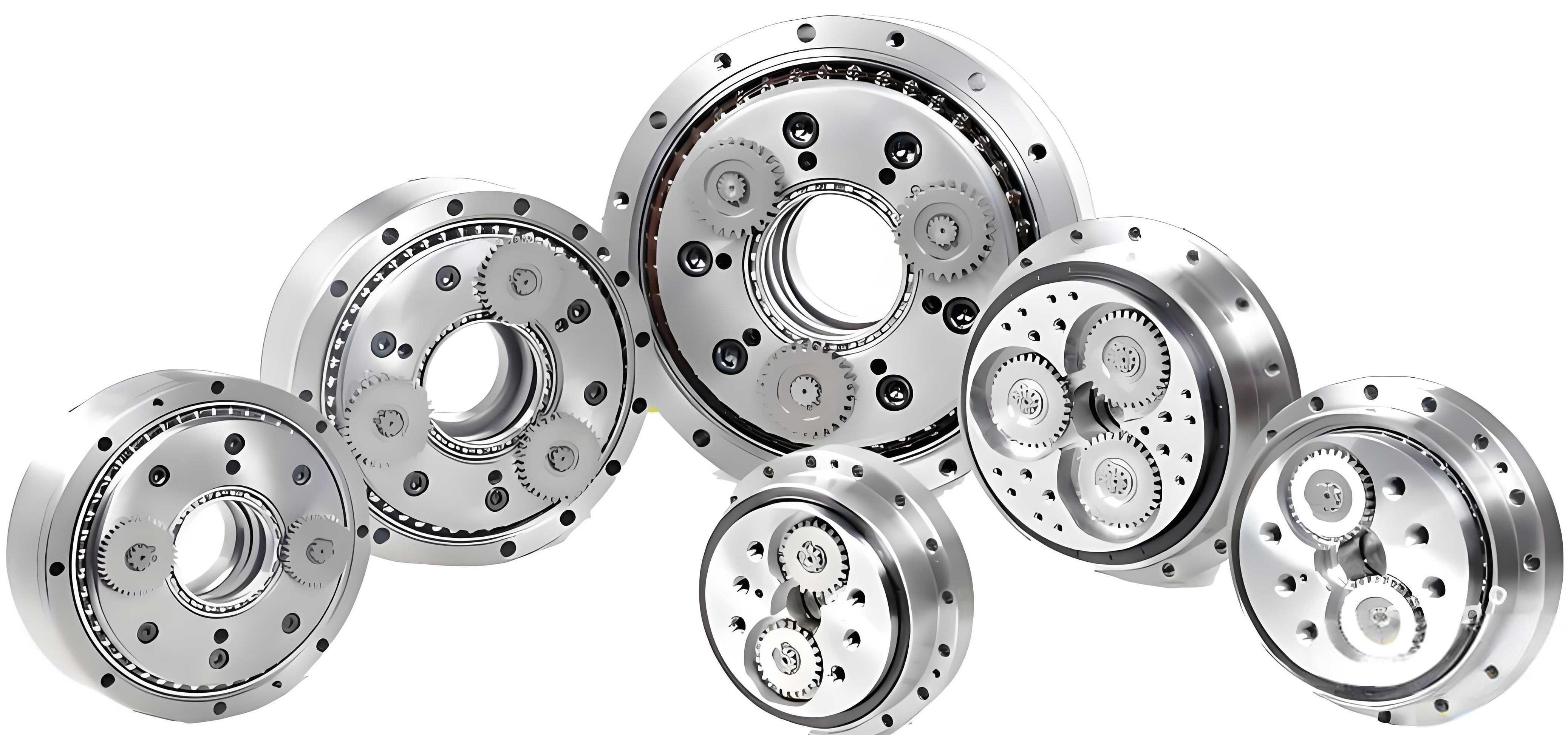
Operating in reciprocating motion adds time-varying speed and load, further complicating the signal and making it more vulnerable to noise contamination, which can obscure crucial fault-related frequency components.
Methodological Foundation and Proposed CAE-GAN Architecture
Theoretical Background of GANs
The foundational Generative Adversarial Network consists of two neural networks, the Generator (G) and the Discriminator (D), engaged in a minimax game. The generator learns to map a random noise vector \(z\) to a data sample \(G(z)\) that resembles the real data distribution \(p_{data}(x)\). The discriminator learns to distinguish between real samples \(x\) and generated (fake) samples \(G(z)\). The original objective function is:
$$
\min_G \max_D V(D, G) = \mathbb{E}_{x \sim p_{data}(x)}[\log D(x)] + \mathbb{E}_{z \sim p_z(z)}[\log(1 – D(G(z)))]
$$
where \(D(x)\) is the discriminator’s probability estimate that \(x\) is real. Training GANs is challenging due to issues like mode collapse and training instability. Several variants have been proposed to mitigate these problems. Conditional GANs (cGANs) provide auxiliary information \(y\) (e.g., the noisy signal) to both generator and discriminator, conditioning the generation process. The Least Squares GAN (LSGAN) replaces the cross-entropy loss with a least squares loss, which provides smoother gradients and helps stabilize training. The loss functions for LSGAN are:
$$
\begin{aligned}
\min_D V(D) &= \mathbb{E}_{x \sim p_{data}(x)}[(D(x) – 1)^2] + \mathbb{E}_{z \sim p_z(z)}[(D(G(z)))^2] \\
\min_G V(G) &= \mathbb{E}_{z \sim p_z(z)}[(D(G(z)) – 1)^2]
\end{aligned}
$$
Our proposed CAE-GAN builds upon these concepts, specifically adapting the cGAN and LSGAN frameworks for the regression task of signal denoising.
Proposed CAE-GAN Model for Denoising
The core innovation lies in the specific design of the generator and discriminator networks and their tailored loss functions for denoising vibration signals from a rotary vector reducer.
Generator Network with Skip Connections
The generator \(G\) is designed as a convolutional auto-encoder (CAE). Its primary function is to take a noisy vibration signal \(\tilde{x}\) as input and output a denoised signal \(\hat{x} = G(\tilde{x})\). The architecture is fully convolutional to preserve the temporal structure and enable input of variable length. The encoder part compresses the input into a latent representation through a series of convolutional layers (with LeakyReLU activation and Batch Normalization), while the decoder part reconstructs the signal from this representation using transposed convolutional layers.
The key architectural improvement is the incorporation of skip connections between corresponding layers in the encoder and decoder. These connections concatenate feature maps from the encoder directly to the decoder at the same resolution level. This allows the network to bypass the bottleneck and directly propagate high-resolution details (like sharp transient features indicative of faults) from the input to the output, addressing the common issue of blurring in auto-encoder based denoising. A schematic representation of this generator is conceptualized as follows:
Generator G: Input(\(\tilde{x}\), 1, L) → [Conv1D→LeakyReLU→BN] → … (Encoder) → Latent Space → … [Deconv1D→LeakyReLU→BN] + Skip Connection → … (Decoder) → Output(\(\hat{x}\), 1, L).
where L is the length of the input signal sample.
Discriminator Network
The discriminator \(D\) is adapted for the denoising task. Instead of judging a single sample, it is designed to judge pairs of signals. It takes two inputs: a reference signal and a target signal. Its job is to determine whether the target signal is the “clean” version of the reference noisy signal. In our framework, it is trained on two types of pairs: 1) a real clean signal \(x\) paired with its corresponding noisy version \(\tilde{x}\) (this pair should be labeled as “real”), and 2) the generator’s denoised output \(\hat{x}\) paired with the same noisy input \(\tilde{x}\) (this pair should be labeled as “fake” during discriminator training). This conditional setup guides the generator to produce outputs that are plausible clean signals given the specific noisy input.
The discriminator is implemented as a deep CNN, ending with a fully connected layer and a sigmoid activation to output a probability score.
Enhanced Loss Functions
The loss functions are critical for stable training and effective denoising. We combine the adversarial loss from LSGAN with a content loss (distance function).
Discriminator Loss (\(L_D\)): The discriminator is trained to assign a score of 1 to (clean, noisy) pairs and 0 to (denoised, noisy) pairs.
$$
\min_D L_D = \mathbb{E}_{x, \tilde{x}}[(D(x, \tilde{x}) – 1)^2] + \mathbb{E}_{\tilde{x}}[(D(G(\tilde{x}), \tilde{x}))^2]
$$
Generator Loss (\(L_G\)): The generator has a two-fold objective: 1) Fool the discriminator, making it assign a high score to its outputs (adversarial loss), and 2) Minimize the distance between its output and the ground-truth clean signal (content loss). We use the L1-norm as the content loss due to its tendency to produce less blurry results than L2-norm.
$$
\min_G L_G = \mathbb{E}_{\tilde{x}}[(D(G(\tilde{x}), \tilde{x}) – 1)^2] + \lambda \cdot \mathbb{E}_{x, \tilde{x}}[||x – G(\tilde{x})||_1]
$$
Here, \(\lambda\) is a hyperparameter that balances the adversarial loss and the content loss. The L1 term \(\|x – \hat{x}\|_1\) directly penalizes deviations from the true clean signal, ensuring perceptual similarity and stabilizing training by providing a strong, direct gradient towards the correct output.
Training Procedure
The training alternates between updating the discriminator and the generator, as summarized in the following process:
- Fix G, update D: Sample a batch of clean-noisy pairs \((x, \tilde{x})\). Generate denoised signals \(\hat{x} = G(\tilde{x})\). Compute \(L_D\) using both \((x, \tilde{x})\) as real and \((\hat{x}, \tilde{x})\) as fake. Update D’s parameters to minimize \(L_D\).
- Fix D, update G: Sample a new batch of noisy signals \(\tilde{x}\). Generate \(\hat{x} = G(\tilde{x})\). Compute \(L_G\) using the current D and the corresponding clean signals \(x\). Update G’s parameters to minimize \(L_G\).
- Repeat steps 1 and 2 until convergence.
Experimental Validation and Analysis
Dataset Description and Experimental Setup
To validate the proposed method, vibration data was collected from a rotary vector reducer test rig simulating industrial robotic joint operation. The setup includes a servo motor driving the rotary vector reducer, which in turn drives a load arm in a 180-degree reciprocating motion. An accelerometer was mounted on the reducer housing. Data was collected under seven distinct health states of the rotary vector reducer, including normal condition and various fault types such as sun gear wear, planet gear wear, and gear root cracks. The raw signals were downsampled to a sampling frequency \(f_s = 512\) Hz. Gaussian white noise at different Signal-to-Noise Ratio (SNR) levels was added to the original signals to simulate harsh industrial acoustic environments.
| State Label | Description | Number of Samples |
|---|---|---|
| S1 | Normal Condition | 500 |
| S2 | Sun Gear Single Flank Wear | 500 |
| S3 | Sun Gear Multiple Flank Wear | 500 |
| S4 | Sun Gear Root Crack | 500 |
| S5 | Planet Gear Single Flank Wear | 500 |
| S6 | Planet Gear Multiple Flank Wear | 500 |
| S7 | Planet Gear Root Crack | 500 |
The performance of the denoising methods was evaluated using two standard metrics calculated between the denoised signal \(\hat{x}\) and the original clean signal \(x\):
- Signal-to-Noise Ratio (SNR) Improvement: \( \text{SNR}_{imp} = 10 \log_{10}\left( \frac{P_{signal}}{P_{error}} \right) \), where \(P_{error}\) is the power of the error signal \((\hat{x} – x)\).
- Mean Squared Error (MSE): \( \text{MSE} = \frac{1}{N}\sum_{i=1}^{N} (\hat{x}_i – x_i)^2 \).
A higher SNR improvement and a lower MSE indicate better denoising performance.
Hyperparameter Selection and Model Configuration
The selection of hyperparameters is crucial for model performance. Key parameters were determined empirically based on the physical characteristics of the rotary vector reducer vibration signals.
Input Sample Length (L): The sample length must be long enough to capture at least one full cycle of the reciprocating motion to contain meaningful fault information. Analysis of the time-domain waveform showed a cycle duration of approximately 3.6 seconds, corresponding to over 1843 sample points at \(f_s = 512\) Hz. A sliding window strategy was used to create fixed-length samples from the continuous signal. Comparative experiments were conducted with different lengths, balancing denoising performance and computational cost.
| Sample Length (L) | Training Time (min) | Average MSE (×10⁻³) | Average SNR Improvement (dB) |
|---|---|---|---|
| 512 | 23.2 | 25.30 | 0.20 |
| 1024 | 23.5 | 10.90 | 5.05 |
| 2048 | 35.7 | 3.48 | 11.31 |
| 4096 | 106.8 | 2.81 | 11.86 |
Based on the results in Table 2, \(L = 2048\) was chosen as the optimal length, providing an excellent trade-off between high denoising performance (low MSE, high SNR) and reasonable training time.
Activation Function Parameter (\(\alpha\)): The generator uses LeakyReLU activation, defined as \(\text{LeakyReLU}(x) = \max(0, x) + \alpha \cdot \min(0, x)\). Since vibration signals contain both positive and negative values, retaining information from negative activations (\(\alpha > 0\)) is important. The parameter \(\alpha\) controls the slope for negative inputs. A grid search was performed to find its optimal value.
| α value | Average MSE (×10⁻³) | Average SNR Improvement (dB) |
|---|---|---|
| 0.01 | 4.21 | 10.15 |
| 0.10 | 3.48 | 11.31 |
| 0.20 | 3.92 | 10.58 |
| 0.30 | 4.05 | 10.42 |
The results in Table 3 indicate that \(\alpha = 0.1\) yields the best performance, and was therefore selected for the final model. Other hyperparameters were set as follows: optimizer = RMSprop (learning rate=0.002), batch size = 32, number of epochs = 100, and the content loss weight \(\lambda = 10\).
Denoising Performance Results and Analysis
The proposed CAE-GAN was trained using the configured parameters. The training process showed stable convergence, with the generator and discriminator losses reaching an equilibrium after approximately 80 epochs. After training, the generator was extracted and used as the denoising model. A sample result for a signal from the test set (with added -10 dB noise) is presented in Figure 1, showing the time-domain waveform and envelope spectrum. The denoised signal from CAE-GAN closely matches the original clean signal, effectively suppressing random noise while preserving the structural characteristics and prominent spectral peaks associated with the rotary vector reducer’s operation.
To quantitatively benchmark the proposed method, it was compared against several traditional and deep learning-based denoising techniques under different input noise levels (-2 dB, -6 dB, -10 dB). The comparison set included:
- Traditional: Singular Value Decomposition (SVD), Empirical Mode Decomposition (EMD).
- Deep Learning: Fully Convolutional Network with Non-Local Blocks (FCN-NLB), Speech Enhancement GAN (SEGAN), and Time-Domain Convolutional GAN (TDC-GAN).
All DL models were trained on the same dataset. The average results over multiple trials are summarized below.
| Method / Noise Level | -2 dB | -6 dB | -10 dB | |||
|---|---|---|---|---|---|---|
| SNRimp (dB) | MSE (×10⁻³) | SNRimp (dB) | MSE (×10⁻³) | SNRimp (dB) | MSE (×10⁻³) | |
| SVD | 8.21 | 9.87 | 7.55 | 11.45 | 6.92 | 13.28 |
| EMD | 9.45 | 7.25 | 8.10 | 9.98 | 7.25 | 12.10 |
| FCN-NLB | 14.32 | 3.85 | 13.88 | 4.21 | 13.05 | 5.08 |
| SEGAN | 15.01 | 3.25 | 14.45 | 3.68 | 13.78 | 4.32 |
| TDC-GAN | 15.88 | 2.65 | 15.15 | 3.08 | 14.25 | 3.85 |
| Proposed CAE-GAN | 17.52 | 1.82 | 17.05 | 2.01 | 16.40 | 2.45 |
The data in Table 4 clearly demonstrates the superiority of the proposed CAE-GAN. It consistently achieves the highest SNR improvement and the lowest MSE across all noise levels. Notably, at the challenging -10 dB noise level, CAE-GAN improves the SNR by over 16 dB, significantly outperforming the next best method (TDC-GAN) by more than 2 dB. This confirms the effectiveness of the architectural enhancements (skip connections) and the hybrid loss function in learning a robust mapping from noisy to clean signals for the rotary vector reducer.
Impact on Fault Diagnosis Accuracy
The ultimate goal of denoising is to improve the reliability of subsequent fault diagnosis. To evaluate this, a separate experiment was conducted. A new dataset of 7000 samples (1000 per fault state) was collected. Different levels of noise were added to create a challenging classification scenario. The trained CAE-GAN generator was used to denoise these signals. Both the original noisy signals and the CAE-GAN-denoised signals were then fed into four different neural network-based fault diagnosis models:
- WDCNN: A deep CNN with wide first-layer kernels.
- TiCNN: A time-invariant CNN model.
- ResNet-18 (1D): A 1D adaptation of the ResNet-18 architecture.
- LeNet-5 (2D): A classic CNN requiring 1D signals to be transformed into 2D spectrograms, potentially losing information.
The classification accuracy was measured for each combination.
| Diagnosis Model | Original (-2 dB) | Original (-6 dB) | Original (-10 dB) | |||
|---|---|---|---|---|---|---|
| Noisy | Denoised | Noisy | Denoised | Noisy | Denoised | |
| WDCNN | 96.73% | 99.50% | 93.99% | 98.73% | 89.13% | 98.41% |
| TiCNN | 97.86% | 99.52% | 95.87% | 99.31% | 91.13% | 98.55% |
| ResNet-18 | 99.36% | 100.00% | 95.50% | 99.90% | 95.06% | 99.72% |
| LeNet-5 (2D) | 93.33% | 97.42% | 88.23% | 94.98% | 84.78% | 92.76% |
The results in Table 5 are compelling. For every diagnostic model and at every noise level, the classification accuracy is substantially higher when using the CAE-GAN-denoised signals compared to the raw noisy signals. The improvement is most dramatic at the highest noise level (-10 dB), where accuracy jumps by approximately 9 percentage points for WDCNN. Furthermore, with denoised inputs, models like WDCNN, TiCNN, and ResNet-18 consistently achieve accuracy above 98%, even when the original signals were severely contaminated. This proves that the proposed denoising method not only improves signal quality metrics but also directly enhances the performance of downstream fault diagnosis systems for the rotary vector reducer by providing cleaner, more discriminative feature representations.
Conclusion
This work presented a novel deep learning-based approach for denoising vibration signals from a rotary vector reducer operating under reciprocating motion. The proposed CAE-GAN model addresses key challenges in GAN training for regression tasks by incorporating a skip-connected convolutional auto-encoder generator and a hybrid loss function combining adversarial and L1-norm content losses. This design stabilizes training, ensures faithful reconstruction of the clean signal’s structure, and effectively suppresses noise while preserving fault-related features.
Experimental validation on a dedicated rotary vector reducer test rig demonstrated the method’s superiority over both traditional techniques (SVD, EMD) and contemporary deep learning denoisers (FCN-NLB, SEGAN, TDC-GAN), as measured by higher SNR improvement and lower MSE. Crucially, the denoised signals significantly boosted the accuracy of multiple neural network-based fault diagnosis models, confirming the practical utility of the method as a preprocessing step for condition monitoring systems.
Future work will focus on deploying the trained CAE-GAN model in an online or edge-computing environment for real-time denoising of vibration data from industrial robots in the field. Further exploration could involve adapting the model to be more robust to varying operational conditions (speed, load) of the rotary vector reducer and investigating its applicability to other complex mechanical components in rotating or reciprocating machinery.