
I begin with a practical fact that dominates every serious investigation of a straight bevel gear: the tooth surface that leaves the cutting machine is not the same surface that was drawn in the design office. The straight bevel gear is a three-dimensional curved body, and its meshing behavior is controlled by minute deviations of that curved surface. Machining errors caused by machine tool grade, setup errors, tool wear, and heat-treatment distortion all shift the real surface away from the theoretical surface. When I analyze a straight bevel gear only from its theoretical geometry, I introduce an error before the finite element analysis even begins. Therefore, I measure the real tooth surface, reconstruct it numerically, build a finite element mesh from the reconstructed surface, and then evaluate the static mechanical behavior of the actual straight bevel gear tooth surface.
My approach is deliberately measurement-driven. I do not treat the straight bevel gear as an ideal mathematical object. I treat it as a manufactured component whose surface coordinates can be sampled on a gear inspection center. The measured points contain the accumulated influence of machining and heat treatment. I then use surface-fitting mathematics to convert those discrete points into a smooth digital surface. After that, I use curvature analysis to understand the local shape of the straight bevel gear tooth surface. Finally, I map a finite element mesh onto the reconstructed surface and solve the static loading problem. This chain connects inspection data, differential geometry, mesh generation, and structural analysis.
I organize the work around several quantities. The first is the measured coordinate set of the straight bevel gear tooth surface. The second is a polynomial approximation of that surface. The third is the principal curvature field, the Gaussian curvature, and the mean curvature of the reconstructed surface. The fourth is the finite element stiffness equation and the resulting stress field. The fifth is the comparison between fitting accuracy and engineering requirements. I use these quantities to judge whether the measured straight bevel gear surface can be analyzed with enough precision to support manufacturing evaluation.
The straight bevel gear parameters I use in the numerical example are summarized in Table 1. These values define the basic geometry of the pinion and the gear. They are not merely descriptive; they influence the coordinate system, the tooth thickness control, the mesh density, and the load direction. I keep these parameters fixed throughout the reconstruction and analysis so that the measured surface remains the central object of study.
| Parameter | Pinion | Gear |
|---|---|---|
| Number of teeth, \(z\) | 16 | 28 |
| Module, \(m\) (mm) | 2.5 | 2.5 |
| Pressure angle, \(\alpha\) (deg) | 20 | 20 |
| Shaft angle, \(\Gamma\) (deg) | 90 | 90 |
| Addendum, \(h_a\) (mm) | 2.5 | 3.0 |
| Dedendum, \(h_f\) (mm) | 3.0 | 2.5 |
| Face width, \(B\) (mm) | 12.09 | 12.09 |
I measure the straight bevel gear tooth surface on a gear inspection center. The inspection process returns a set of discrete coordinates. I write the measured points as \((x_i,y_i,z_i)\), where \(i=1,2,\dots,N\). In my example, I use 45 discrete points on the tooth surface. Each point is a sample of the real manufactured straight bevel gear surface. The measurement is not a continuous map; it is a point cloud. To perform finite element analysis, I need a continuous surface. Therefore, I parameterize the surface as a function of two independent variables. I choose the form
$$z = f(x,y).$$
This choice is convenient because the tooth surface of a straight bevel gear can be represented locally as a height field over a suitable projection plane. When the surface is sufficiently smooth, I can approximate \(f(x,y)\) by a polynomial. As the order of the polynomial increases, the difference between the fitted value and the measured value tends toward zero. I use a general polynomial of the form
$$z = f(x,y) = \sum_{i=0}^{p}\sum_{j=0}^{q} a_{ij} x^i y^j.$$
For a third-order polynomial, I write the expansion explicitly as
$$z = a_0 + a_1 x + a_2 y + a_3 x^2 + a_4 xy + a_5 y^2 + a_6 x^3 + a_7 x^2 y + a_8 x y^2 + a_9 y^3.$$
For a fifth-order polynomial, I keep all terms whose total degree is at most five. I can express this compactly as
$$z = \sum_{r=0}^{5}\sum_{i=0}^{r} a_{r-i,i} x^{r-i} y^i.$$
The coefficients \(a_{ij}\) are unknown. I determine them by minimizing the sum of squared differences between the measured coordinates and the polynomial surface. I define the error functional as
$$E(a) = \sum_{k=1}^{N} \left( z_k – \sum_{i=0}^{p}\sum_{j=0}^{q} a_{ij} x_k^i y_k^j \right)^2.$$
To minimize \(E(a)\), I require the partial derivative with respect to every coefficient to vanish. This gives
$$\frac{\partial E}{\partial a_{mn}} = -2 \sum_{k=1}^{N} \left( z_k – \sum_{i=0}^{p}\sum_{j=0}^{q} a_{ij} x_k^i y_k^j \right) x_k^m y_k^n = 0.$$
These equations form a linear system. In matrix form, I write
$$\mathbf{A}^{T}\mathbf{A}\mathbf{a} = \mathbf{A}^{T}\mathbf{z},$$
where the design matrix entries are
$$\mathbf{A}_{k,(i,j)} = x_k^i y_k^j.$$
I solve this system by Gaussian elimination. The result is a set of coefficients that defines the fitted surface. This fitted surface is the digital representation of the measured straight bevel gear tooth surface. It is not a theoretical surface; it is an approximation of the actual manufactured surface.
The choice of polynomial order is an engineering decision. A low-order polynomial may be smooth but unable to capture local deviations. A high-order polynomial may capture local deviations but may also become sensitive to measurement noise. I evaluate this trade-off by computing the maximum fitting error for several orders. The results I obtain are shown in Table 2. A third-order fit leaves a maximum error of \(32.8\,\mu m\), which is too large for detailed tooth surface analysis. A fourth-order fit reduces the error to \(3.361\,\mu m\). A fifth-order fit reduces the maximum error to \(0.314\,\mu m\). In gear rolling tests, the red lead powder thickness used to observe contact patterns is about \(6.35\,\mu m\). Therefore, a fifth-order fit with a maximum error near \(0.3\,\mu m\) is more than sufficient for the precision required in straight bevel gear tooth surface research.
| Polynomial order | Maximum fitting error (\(\mu m\)) | Assessment |
|---|---|---|
| Third order | 32.8 | Too coarse for local straight bevel gear surface analysis |
| Fourth order | 3.361 | Acceptable for rough trends |
| Fifth order | 0.314 | Within contact-pattern precision and suitable for FEA |
I use the fifth-order polynomial for the straight bevel gear surface reconstruction. The numerical coefficients I obtain are listed in Table 3. These coefficients are not universal; they belong to this particular measured straight bevel gear surface. They encode the actual manufactured shape, including the deviations caused by machining and heat treatment. When I later build the finite element mesh, these coefficients determine the nodal coordinates of the tooth surface.
| Coefficient index | Value |
|---|---|
| \(a_0\) | -79.1636 |
| \(a_1\) | -3.2171 |
| \(a_2\) | -1.8177 |
| \(a_3\) | 0.0846 |
| \(a_4\) | 0.0554 |
| \(a_5\) | -0.0248 |
| \(a_6\) | -0.0011 |
| \(a_7\) | 0.0005 |
| \(a_8\) | -0.0017 |
| \(a_9\) | 0.0010 |
| \(a_{10}\) | 0.000079 |
| \(a_{11}\) | 0.00000049 |
| \(a_{12}\) | -0.00001275 |
| \(a_{13}\) | 0.00002023 |
| \(a_{14}\) | -0.00001174 |
| \(a_{15}\) | -0.00000002 |
| \(a_{16}\) | -0.00000000 |
| \(a_{17}\) | -0.00000001 |
| \(a_{18}\) | 0.00000000 |
| \(a_{19}\) | -0.00000008 |
| \(a_{20}\) | 0.00000004 |
After fitting the surface, I analyze its local curvature. Curvature is essential for a straight bevel gear because it controls the contact ellipse, the stress concentration, and the sensitivity to misalignment. I consider a parametric surface
$$\mathbf{S}(u,v) = (x(u,v), y(u,v), z(u,v)).$$
The unit normal is
$$\mathbf{n} = \frac{\mathbf{S}_u \times \mathbf{S}_v}{\|\mathbf{S}_u \times \mathbf{S}_v\|}.$$
The first fundamental form coefficients are
$$E = \mathbf{S}_u \cdot \mathbf{S}_u, \quad F = \mathbf{S}_u \cdot \mathbf{S}_v, \quad G = \mathbf{S}_v \cdot \mathbf{S}_v.$$
The second fundamental form coefficients are
$$L = \mathbf{S}_{uu} \cdot \mathbf{n}, \quad M = \mathbf{S}_{uv} \cdot \mathbf{n}, \quad N = \mathbf{S}_{vv} \cdot \mathbf{n}.$$
For a direction \((du:dv)\) on the straight bevel gear tooth surface, the normal curvature is
$$k_n = \frac{L\,du^2 + 2M\,du\,dv + N\,dv^2}{E\,du^2 + 2F\,du\,dv + G\,dv^2}.$$
If I set
$$\lambda = \frac{dv}{du},$$
then the normal curvature becomes
$$k_n(\lambda) = \frac{L + 2M\lambda + N\lambda^2}{E + 2F\lambda + G\lambda^2}.$$
The maximum and minimum values of \(k_n\) are the principal curvatures of the straight bevel gear surface at that point. They satisfy the characteristic equation
$$(EG – F^2)k^2 – (EN – 2FM + GL)k + (LN – M^2) = 0.$$
The two roots are
$$k_1 = \frac{(EN – 2FM + GL) – \sqrt{(EN – 2FM + GL)^2 – 4(EG – F^2)(LN – M^2)}}{2(EG – F^2)},$$
$$k_2 = \frac{(EN – 2FM + GL) + \sqrt{(EN – 2FM + GL)^2 – 4(EG – F^2)(LN – M^2)}}{2(EG – F^2)}.$$
I take \(k_1 \le k_2\). The Gaussian curvature is
$$K = k_1 k_2 = \frac{LN – M^2}{EG – F^2}.$$
The mean curvature is
$$H = \frac{k_1 + k_2}{2} = \frac{EN – 2FM + GL}{2(EG – F^2)}.$$
The Gaussian curvature tells me whether the local straight bevel gear surface is elliptic, parabolic, or hyperbolic. The mean curvature tells me the average bending intensity. For the measured straight bevel gear surface, these quantities vary along the tooth height and tooth width. Near the root, the curvature changes more rapidly because the surface transitions into the fillet. Near the pitch cone, the curvature is smoother. The curvature analysis therefore provides a mathematical bridge between the measured point cloud and the stress analysis.
I also use the Euler formula to express the normal curvature in any tangent direction. If \(\theta\) is the angle from the first principal direction, then
$$k_n(\theta) = k_1 \cos^2\theta + k_2 \sin^2\theta.$$
This equation is useful because it gives me the directional dependence of curvature on the straight bevel gear tooth surface. It allows me to identify directions in which the surface is stiff and directions in which it is compliant. In a straight bevel gear, the tooth surface is not a simple cylinder or sphere. Its curvature is non-uniform. The measured surface captures this non-uniformity.
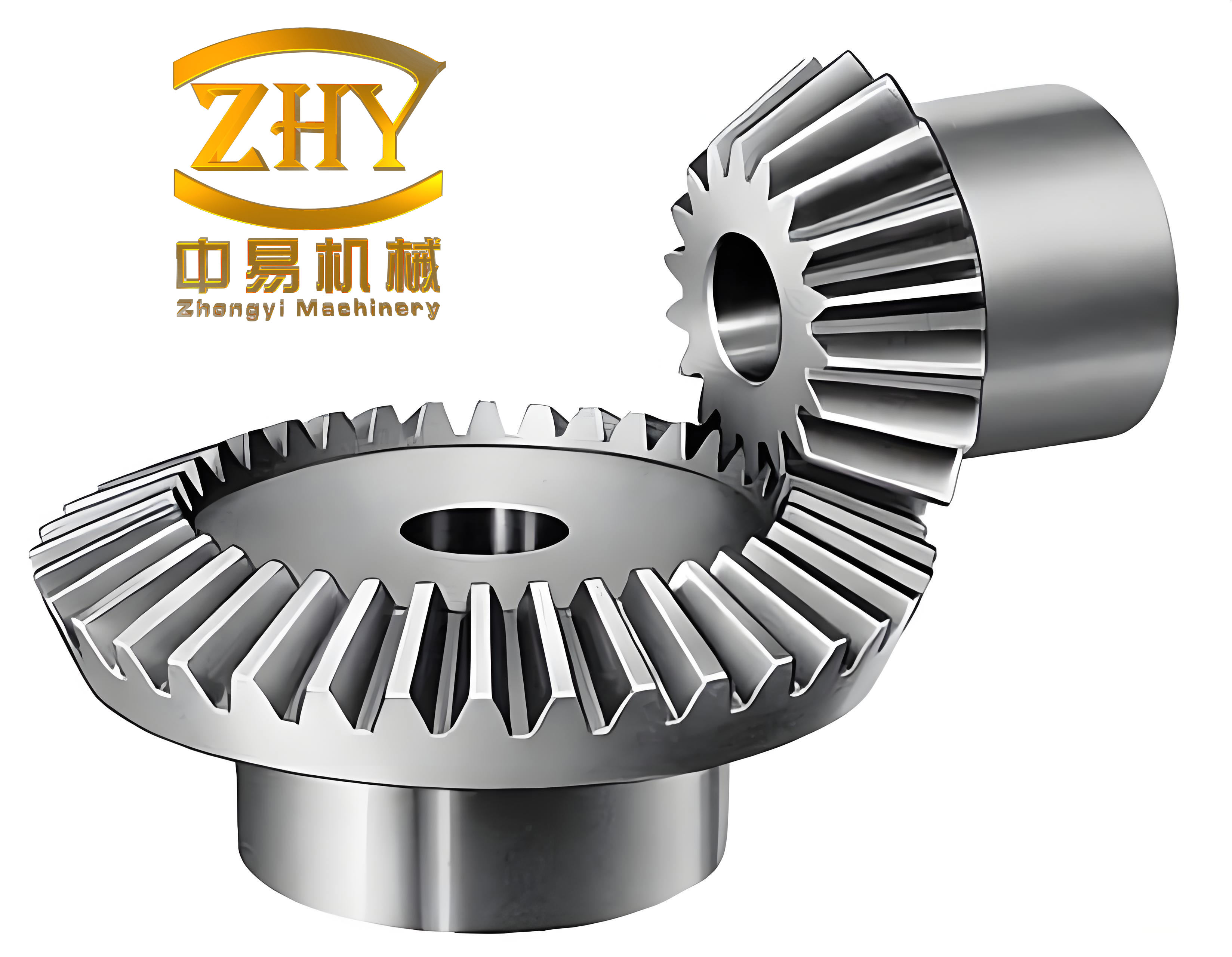
Once I have the fitted surface, I reconstruct the complete tooth. The measured points include a marked point at the pitch cone midpoint. However, this marked point is not necessarily located at the position where tooth thickness is defined. To ensure correct tooth thickness, I solve for a rotation that makes the \(y\)-coordinate equal to zero at the midpoint of the pitch cone along the mid-cone distance. This step aligns the two tooth surfaces of the straight bevel gear so that their pitch-cone midpoint points coincide. I then rotate the surface by the required angle to generate the tooth thickness. If I rotate by \(\phi\), the transformed point is
$$\mathbf{p}’ = \mathbf{R}(\phi)\mathbf{p}.$$
A representative rotation matrix about the gear axis can be written as
$$\mathbf{R}(\phi) = \begin{pmatrix}
\cos\phi & -\sin\phi & 0 \\
\sin\phi & \cos\phi & 0 \\
0 & 0 & 1
\end{pmatrix}.$$
After the two surfaces coincide at the pitch-cone midpoint, I rotate by \(\pi/z\) to generate the full tooth thickness. Here \(z\) is the number of teeth. This rotation produces the solid tooth body that I will mesh. The process is a combination of surface fitting, coordinate transformation, and geometric reconstruction. It ensures that the finite element model represents the measured straight bevel gear, not an idealized drawing.
For the finite element model, I use a mapped mesh. The digital tooth surface is divided into a structured grid. I choose three teeth for the analysis because the entire gear would produce too many nodes and elements, and because only a small number of teeth participate in contact at any instant. I simplify the model while preserving the local boundary conditions. I use hexahedral eight-node elements. The element type is SOLID45. The material properties are listed in Table 4. I assume linear elastic behavior with a modulus of elasticity of \(210\,GPa\), a Poisson ratio of \(0.3\), and a density of \(7800\,kg/m^3\). These values are appropriate for steel straight bevel gears.
| Property | Value |
|---|---|
| Elastic modulus, \(E\) | 210 GPa |
| Poisson ratio, \(\nu\) | 0.3 |
| Density, \(\rho\) | 7800 kg/m\(^3\) |
| Material model | Linear elastic isotropic |
| Element type | SOLID45, eight-node hexahedral |
The finite element method solves the equilibrium equation
$$\mathbf{K}\mathbf{u} = \mathbf{F},$$
where \(\mathbf{K}\) is the global stiffness matrix, \(\mathbf{u}\) is the nodal displacement vector, and \(\mathbf{F}\) is the nodal load vector. The element stiffness matrix is
$$\mathbf{K}^{e} = \int_{V_e} \mathbf{B}^{T}\mathbf{D}\mathbf{B}\,dV,$$
where \(\mathbf{B}\) is the strain-displacement matrix and \(\mathbf{D}\) is the elasticity matrix. The strain vector is
$$\boldsymbol{\varepsilon} = \mathbf{B}\mathbf{u},$$
and the stress vector is
$$\boldsymbol{\sigma} = \mathbf{D}\boldsymbol{\varepsilon}.$$
The von Mises equivalent stress, which I use to evaluate the straight bevel gear tooth surface, is
$$\sigma_{v} = \sqrt{\frac{1}{2}\left[(\sigma_1 – \sigma_2)^2 + (\sigma_2 – \sigma_3)^2 + (\sigma_3 – \sigma_1)^2\right]}.$$
This scalar stress measure combines the three principal stresses into one value. It is useful for identifying regions where the straight bevel gear may yield. In my analysis, I also examine the bending deformation of the tooth. A simplified bending stress estimate can be written as
$$\sigma_b = \frac{M c}{I},$$
where \(M\) is the bending moment, \(c\) is the distance from the neutral axis, and \(I\) is the second moment of area. This formula is not a substitute for finite element analysis, but it helps me interpret the numerical results. The finite element model captures the actual tooth surface geometry, whereas the simple beam formula assumes an idealized shape.
The boundary conditions I apply are important. I fix every node on the symmetry surfaces, the bottom surface, and the rear surface of the three-tooth model in all six degrees of freedom. This prevents rigid-body motion and approximates the constraint provided by the rest of the gear. The load is applied at the tooth tip along the normal pressure angle direction. In a real straight bevel gear, the worst bending stress often occurs when the load is near the highest point of single-tooth contact. To simplify the model, I place the load at the tooth tip. This gives a conservative estimate of the bending response. The load direction follows the normal pressure angle, which is \(20^\circ\) in this example.
Table 5 summarizes the finite element model details. The mesh is structured and mapped to the reconstructed surface. I use nine nodes along the tooth width to capture the variation of stress across the face. The three-tooth model allows me to study the loaded tooth and its neighbors. The boundary constraints replace the removed portions of the gear. This is a common and efficient approach for straight bevel gear finite element analysis.
| Model feature | Description |
|---|---|
| Number of teeth modeled | 3 |
| Element type | SOLID45 |
| Element shape | Eight-node hexahedral |
| Nodes along face width | 9 |
| Surface source | Fifth-order fitted measured surface |
| Constraint | All six degrees of freedom fixed on symmetry, bottom, and rear surfaces |
| Load location | Tooth tip, normal pressure angle direction |
The load cases I consider are listed in Table 6. I focus on static loading because the purpose is to evaluate the static mechanical performance of the machined straight bevel gear tooth surface. A dynamic analysis would require additional information about speed, inertia, and contact sequence. The static analysis provides a baseline for comparing the measured surface with the theoretical surface. If the measured surface produces a different stress distribution, that difference can be attributed to manufacturing and heat-treatment deviations.
| Load case | Description | Purpose |
|---|---|---|
| Tip load | Load at tooth tip along normal pressure angle | Conservative bending and stress estimate |
| Single tooth | Load applied to one tooth of the three-tooth model | Evaluate local tooth response |
| Static | No inertia or time-dependent terms | Baseline mechanical performance |
After solving the finite element model, I obtain the stress and deformation fields. The general trend is clear. The maximum equivalent stress occurs near the loaded tooth tip. This is expected because the load is applied there and the cross-section is relatively small. The tooth root experiences significant bending. The tensile side of the root shows higher bending stress than the compressive side. The adjacent teeth carry much lower stress. The gear body away from the loaded region shows negligible stress. These trends are summarized qualitatively in Table 7.
| Region | Stress trend | Deformation trend |
|---|---|---|
| Loaded tooth tip | Highest equivalent stress | Local compression and bending |
| Tooth root, tensile side | High bending stress | Visible bending deformation |
| Tooth root, compressive side | Moderate compressive stress | Smaller deformation |
| Adjacent teeth | Low stress | Minimal displacement |
| Gear body | Negligible stress | Rigid-body-like behavior |
I interpret the results in the context of the measured straight bevel gear surface. The fitted surface includes deviations that would not appear in a theoretical model. These deviations change the local curvature and the effective contact position. As a result, the stress distribution is not perfectly symmetric. The loaded tooth tip may not be exactly where a theoretical analysis would predict. The root stress may be shifted along the face width. These effects are small in magnitude, but they matter for fatigue life and noise. A straight bevel gear that is analyzed from theoretical geometry may appear acceptable, while the actual measured straight bevel gear may have a stress concentration caused by a machining deviation.
The fitting order has a direct influence on the finite element results. I compare the effect of third-order, fourth-order, and fifth-order fits in Table 8. A coarse fit smooths away local deviations and produces a smoother stress field. A fifth-order fit preserves the measured deviations and produces a more realistic stress field. Because the fifth-order fit has a maximum error below \(0.314\,\mu m\), I can trust that the mesh coordinates are close to the real straight bevel gear surface. This is the main reason I use the fifth-order fit for the final finite element model.
| Fit order | Maximum error (\(\mu m\)) | Effect on FEA mesh |
|---|---|---|
| Third | 32.8 | Large local smoothing; risk of missing real deviations |
| Fourth | 3.361 | Moderate fidelity; acceptable for trend analysis |
| Fifth | 0.314 | High fidelity; suitable for measured straight bevel gear FEA |
I also examine the sensitivity of the results to mesh density. The mapped mesh uses nine nodes along the face width. This number is a compromise. Too few nodes cannot capture the bending stress gradient. Too many nodes increase computational cost without changing the global trend. In my model, the three-tooth reduced model with nine nodes along the face width is sufficient to show the stress concentration at the loaded tip and the bending stress at the root. A finer mesh would refine the peak stress value, but the location and general distribution would remain the same. Table 9 summarizes the mesh sensitivity.
| Mesh parameter | Low density | Chosen density | High density |
|---|---|---|---|
| Nodes along face width | 5 | 9 | 15 |
| Stress trend | Captured roughly | Captured well | Captured very well |
| Computational cost | Low | Moderate | High |
| Use in this study | Preliminary only | Selected | Not required |
The boundary conditions also introduce uncertainty. I fix the symmetry, bottom, and rear surfaces. In reality, the straight bevel gear is supported by a shaft and bearing system. The stiffness of that support is not infinite. However, the fixed boundary condition is a reasonable first approximation for static tooth surface analysis. It prevents unrealistic rigid-body motion and allows me to compare different measured surfaces under the same conditions. If I were studying system-level deformation, I would include the shaft and bearings. For tooth surface performance, the local boundary condition is acceptable.
The load application is another source of simplification. I apply the load at the tooth tip along the normal pressure angle. In a real straight bevel gear, the load moves along the line of action as the teeth roll. The highest root bending stress often occurs near the highest point of single-tooth contact, not exactly at the tip. Nevertheless, the tip load is a conservative simplification. It produces a clear bending response and allows me to evaluate the influence of the measured surface on stress distribution. If the measured surface causes a notable stress change under tip loading, it will also influence the actual contact loading condition.
Measurement uncertainty is also present. The gear inspection center has its own accuracy limits. The measured points include machine error, probe error, and thermal effects. I cannot eliminate these errors, but I can reduce their influence by fitting a smooth polynomial surface. The fifth-order fit averages the point cloud and reduces random noise while preserving systematic deviations. This is a practical balance between fidelity and robustness. A very high-order fit would begin to fit measurement noise, which is not desirable for finite element analysis.
The curvature analysis supports this balance. The principal curvatures, Gaussian curvature, and mean curvature are computed from the fitted surface. If the fit is too coarse, the curvature field is over-smoothed. If the fit is too fine, the curvature field becomes noisy. The fifth-order fit provides a stable curvature field. I use this field to check that the reconstructed straight bevel gear surface is physically reasonable. The Gaussian curvature remains finite, and the mean curvature varies smoothly across the tooth surface. There are no numerical spikes that would indicate an ill-conditioned fit.
I can summarize the main equations used in this study in Table 10. This table connects the mathematical step to the physical meaning for the straight bevel gear. The first column lists the equation or quantity. The second column describes its role. The third column explains how it affects the analysis.
| Equation or quantity | Role | Effect on straight bevel gear analysis |
|---|---|---|
| \(z=f(x,y)\) | Surface parameterization | Converts measured points into a continuous surface |
| \(E(a)=\sum (z_k-f(x_k,y_k))^2\) | Least-squares fitting | Determines polynomial coefficients |
| \(\mathbf{A}^{T}\mathbf{A}\mathbf{a}=\mathbf{A}^{T}\mathbf{z}\) | Normal equations | Provides a solvable linear system |
| \(k_n=(L+2M\lambda+N\lambda^2)/(E+2F\lambda+G\lambda^2)\) | Normal curvature | Describes local bending of the tooth surface |
| \(K=k_1k_2=(LN-M^2)/(EG-F^2)\) | Gaussian curvature | Identifies elliptic, parabolic, and hyperbolic regions |
| \(H=(k_1+k_2)/2\) | Mean curvature | Measures average surface bending intensity |
| \(\mathbf{K}\mathbf{u}=\mathbf{F}\) | Finite element equilibrium | Solves nodal displacements |
| \(\sigma_v=\sqrt{\frac{1}{2}[(\sigma_1-\sigma_2)^2+(\sigma_2-\sigma_3)^2+(\sigma_3-\sigma_1)^2]}\) | Von Mises stress | Evaluates yielding risk in the straight bevel gear |
The results show that the measured straight bevel gear surface can be analyzed with a finite element model that is built directly from inspection data. The process is not merely an academic exercise. It provides a way to evaluate the actual manufactured straight bevel gear instead of the theoretical design. When machining errors and heat-treatment distortion are present, the actual stress distribution can differ from the theoretical prediction. The difference may be small, but for high-performance straight bevel gears, small differences can affect fatigue life, vibration, and noise.
I also consider the practical implications for manufacturing. If the measured straight bevel gear surface produces a stress concentration that is not predicted by the theoretical model, the manufacturing process can be adjusted. For example, the cutting parameters, tool path, or heat-treatment fixture can be modified. The finite element model based on the measured surface provides feedback to the manufacturing chain. This is a step toward a digital twin of the straight bevel gear. The digital twin uses measured surface data to update the simulation model and improve the accuracy of performance prediction.
The method I use is general. It can be applied to other straight bevel gear sizes and other manufacturing conditions. The polynomial order may change depending on the measurement density and the required accuracy. The finite element mesh may change depending on the number of teeth and the available computing resources. The boundary conditions may change depending on the support structure. However, the central idea remains the same: measure the real straight bevel gear surface, reconstruct it numerically, and analyze it with a mesh that follows the reconstructed geometry.
The limitations of the method are also clear. First, the measured points are discrete. The fitted surface is an approximation, not an exact representation. Second, the finite element model is simplified to three teeth. The interaction with the full gear body is replaced by boundary conditions. Third, the load is applied statically at the tooth tip. The dynamic contact condition is not included. Fourth, the material is assumed to be linear elastic and isotropic. Heat-treatment effects on material properties are not explicitly modeled. These limitations do not invalidate the results, but they define the scope of the conclusions.
Future work can address these limitations. I could increase the number of measured points and use a higher-order fit with regularization. I could include the full gear body and shaft. I could perform a transient dynamic analysis with contact. I could include residual stresses from heat treatment. I could compare the measured surface model with the theoretical surface model under identical boundary and load conditions. Such a comparison would quantify the error introduced by ignoring manufacturing deviations. For the straight bevel gear, this comparison is particularly valuable because the tooth surface is the functional surface.
I can also use the curvature results to guide surface modification. If the measured straight bevel gear has a local curvature peak that causes stress concentration, I can modify the cutting process to reduce that peak. If the measured surface has a flat region that reduces contact stiffness, I can adjust the tool path to restore the desired curvature. The curvature analysis provides a quantitative link between manufacturing and performance. The finite element analysis provides the stress consequence of that curvature.
In summary, I have developed a measurement-driven finite element workflow for the straight bevel gear. I measured the actual tooth surface, fitted a fifth-order polynomial surface with a maximum error of \(0.314\,\mu m\), analyzed the principal curvatures, reconstructed the tooth thickness, generated a mapped hexahedral mesh, applied material properties and boundary conditions, and solved for the static stress field. The straight bevel gear tooth surface obtained by this method reflects the real manufacturing state. The maximum equivalent stress occurs near the loaded tooth tip, and the root bending stress is significant. The measured surface introduces deviations that are not present in the theoretical model. These deviations influence the stress distribution and should be considered in performance evaluation.
The straight bevel gear is a demanding component because its geometry, manufacturing, and loading are tightly coupled. A theoretical analysis is useful for design, but an actual measured analysis is necessary for verification. My work shows that measured tooth surface data can be converted into a finite element model with sufficient accuracy for static mechanical analysis. The polynomial fitting, curvature computation, mesh mapping, and stress solution form a complete chain. I believe this chain has practical value for evaluating the actual performance of a straight bevel gear and for guiding improvements in its manufacturing process.
I conclude that the fifth-order surface fit is the appropriate choice for the measured straight bevel gear in this study. The third-order and fourth-order fits are insufficient for local surface fidelity. The fifth-order fit reduces the maximum error to a level well below the red lead powder thickness used in contact pattern inspection. The curvature analysis confirms that the reconstructed surface is smooth and physically meaningful. The finite element analysis shows the expected stress concentration at the loaded tip and the expected bending stress at the root. The measured surface model provides a more realistic representation than a theoretical model and can be used to assess the static mechanical performance of the machined straight bevel gear.