
Modern transmission systems increasingly demand compact architectures, high-precision motion, and adjustable backlash. To address these requirements, I propose an internal helical planar enveloping screw gear drive. This screw gear concept combines the advantages of internal meshing with a planar enveloping worm profile, resulting in a screw gear pair that is more compact, more precise, and more adjustable than conventional cylindrical worm drives. In this work, I systematically investigate the meshing theory, performance characteristics, parameter optimization, and three-dimensional modeling of this internal helical screw gear drive. The screw gear is treated as a conjugated pair in which the worm surface is generated by a planar internal gear. I derive the meshing functions, contact line equations, boundary curves, and key meshing parameters for both forward and reverse rotations. I then analyze the influence of major design parameters on macro- and micro-meshing behavior. Based on these results, I establish a multi-objective nonlinear optimization model and solve it using the fmincon algorithm. Finally, I build a solid model and perform an interference check to validate the design. The proposed screw gear drive offers a promising solution for robotic joint reducers and other precision transmission applications.
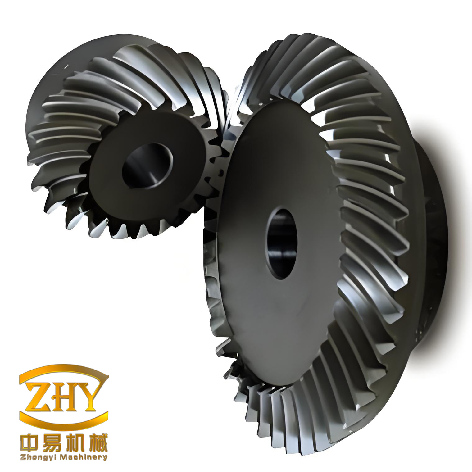
1. Geometric Framework and Moving Frames
I establish a moving frame system to describe the relative motion between the internal helical screw gear and the worm. The screw gear pair operates under orthogonal axes. The base frames are denoted by $$\sigma^{(m)}$$ and $$\sigma^{(n)}$$, which represent the initial positions of the worm and the internal gear, respectively. The worm axis coincides with $$z_m$$, and the internal gear axis coincides with $$z_n$$. The center distance between these axes is $$A$$. The moving frames $$\sigma^{(1)}$$, $$\sigma^{(2)}$$, and $$\sigma^{(3)}$$ are attached to the worm, the internal gear, and the auxiliary reference, respectively. The angular velocities satisfy $$\omega_2 = \omega_3$$, and the transmission ratio is defined as $$i_{12} = \omega_1 / \omega_2$$.
For the forward rotation, which I call side A, the working frame is $$\sigma^{(p)}$$ with origin $$O_p$$ at the intersection of the base circle and the coordinate axis. The coordinate $$x_p$$ is tangent to the base circle, $$y_p$$ is aligned with the generatrix, and the angle between $$z_p$$ and $$x_p$$ is the母平面倾角, or inclination angle, $$\beta$$. The rotation angles are related by
$$\begin{cases}
\varphi_1 = \omega_1 t \\
\varphi_2 = \omega_2 t \\
\varphi_3 = \pi – \theta + \varphi_2
\end{cases}$$
where $$\theta$$ is the angular position of the base circle tangent point. For the reverse rotation, which I call side B, the worm rotates in the opposite direction. The working frame is $$\sigma^{(q)}$$, and the corresponding angles satisfy
$$\begin{cases}
\varphi_2 = \omega_2 t \\
\varphi_3 = \pi – \theta + \varphi_2 \\
\varphi_1′ = i_{12} (\pi – \theta + \varphi_3)
\end{cases}$$
The geometric relationship between side A and side B is symmetric about the worm mid-plane. This symmetry allows me to analyze only side A in detail and then apply the results to side B. The basic geometric parameters of the screw gear pair are summarized in Table 1.
| Parameter | Symbol | Value |
|---|---|---|
| Module in the mid-plane | $$m_t$$ | 4 mm |
| Base circle radius | $$r_b$$ | 62.5 mm |
| Inclination angle | $$\beta$$ | 19.5° |
| Center distance | $$A$$ | 100 mm |
| Number of worm starts | $$z_1$$ | 1 |
| Number of internal gear teeth | $$z_2$$ | 80 |
| Number of engaged teeth | $$z’$$ | 4 |
| Face width | $$B$$ | 110 mm |
The position of the meshing point on side A is expressed in the working frame as $$P(u_3, v_3, 0)$$. The coordinates in the auxiliary frame $$\sigma^{(3)}$$ are
$$\begin{cases}
x_3 = v_3 \sin\beta + r_b \\
y_3 = u_3 \\
z_3 = v_3 \cos\beta
\end{cases}$$
For side B, the meshing point is $$Q(u_2, v_2, 0)$$, and its coordinates in $$\sigma^{(2)}$$ are
$$\begin{cases}
x_2 = v_2 \sin\beta + r_b \\
y_2 = -u_2 \\
z_2 = v_2 \cos\beta
\end{cases}$$
These coordinate transformations form the basis for deriving the meshing functions and contact line equations of the screw gear pair.
2. Meshing Functions and Contact Line Equations
Using the moving frame method, I derive the relative velocity between the worm and the internal gear. For side A, the relative velocity $$v^{(31)}_p$$ in the working frame is expressed as
$$v^{(31)}_p = v^{(31)}_x i_3 + v^{(31)}_y j_3 + v^{(31)}_z k_3$$
where the components are
$$\begin{aligned}
v^{(31)}_x &= \omega_1 \left[ (i_{21} \sin\delta – u_3) \cos\beta + A \sin\varphi_3 \sin\delta \right] \\
v^{(31)}_y &= \omega_1 \left[ (i_{21} \sin\delta – v_3 \sin\beta + r_b) \cos\varphi_3 – A \cos\delta \sin\varphi_3 \right] \\
v^{(31)}_z &= \omega_1 \left[ (v_3 \sin\beta – r_b) \sin\varphi_3 \cos\delta – u_3 \cos\varphi_3 \cos\delta – A \cos\delta \right]
\end{aligned}$$
The meshing function for side A, denoted by $$\Phi^{(3)}$$, is obtained from the dot product of the normal vector and the relative velocity:
$$\Phi^{(3)} = n^{(3)} \cdot v^{(31)}_p = 0$$
Substituting the normal vector $$n^{(3)} = \cos\beta i_3 + \sin\beta k_3$$ and the velocity components yields
$$\begin{aligned}
\Phi^{(3)} = &\; \omega_1 \left[ (i_{21} \sin\delta – u_3) \cos\beta \cos\varphi_3 \right. \\
& + \left. (v_3 \sin\beta – r_b) \sin\varphi_3 \cos\delta \cos\beta \right. \\
& + \left. (v_3 \sin\beta – r_b) \cos\varphi_3 \sin\beta \right. \\
& + \left. A \sin\delta \cos\beta \cos\varphi_3 – A \cos\delta \sin\beta \right]
\end{aligned}$$
Solving $$\Phi^{(3)} = 0$$ for $$v_3$$ as a function of $$u_3$$ and $$\varphi_3$$ gives the contact line equation for side A:
$$v_3 = \frac{(i_{21} \sin\delta – u_3) \cos\beta \cos\varphi_3 + A \sin\delta \cos\beta \cos\varphi_3 – A \cos\delta \sin\beta}{( \sin\beta \sin\varphi_3 \cos\delta + \cos\varphi_3 \sin\beta ) \cos\beta + \sin\beta \cos\varphi_3 \sin\beta}$$
For side B, the relative velocity $$v^{(21)}_q$$ is derived analogously. The meshing function $$\Phi^{(2)}$$ is
$$\Phi^{(2)} = n^{(2)} \cdot v^{(21)}_q = 0$$
and the corresponding contact line equation is
$$v_2 = \frac{(i_{21} \sin\delta – u_2) \cos\beta \cos\varphi_2 + A \sin\delta \cos\beta \cos\varphi_2 + A \cos\delta \sin\beta}{( \sin\beta \sin\varphi_2 \cos\delta + \cos\varphi_2 \sin\beta ) \cos\beta – \sin\beta \cos\varphi_2 \sin\beta}$$
These contact line equations describe the instantaneous contact curves on the screw gear tooth surface. They are essential for evaluating the macroscopic meshing performance, such as contact area and load distribution.
3. Boundary Curves
I derive two types of boundary curves for the internal helical screw gear drive. The second kind boundary curve, also called the meshing limit curve, is obtained by combining the meshing function and its time derivative:
$$\begin{cases}
\Phi^{(i)} = 0 \\
\Phi_t^{(i)} = 0
\end{cases}$$
For side A, the second kind boundary function is
$$\Phi_t^{(3)} = \omega_1 \left[ \cos\varphi_3 \cos\delta \cos\beta – \sin\varphi_3 \sin\delta \cos\beta – \sin\varphi_3 \sin\delta \right] = 0$$
Together with the contact line equation, this yields the second kind boundary curve on the screw gear surface. The first kind boundary curve, also known as the undercutting limit curve, is obtained from
$$\begin{cases}
\Psi^{(i)} = 0 \\
\Phi^{(i)} = 0
\end{cases}$$
where $$\Psi^{(i)}$$ is defined by the first and second fundamental quantities of the surface. For side A, the first kind boundary function is
$$\Psi^{(3)} = \frac{1}{D^{(3)}} \left[ E^{(3)} \Phi_{u_3}^{(3)} \Phi_{v_3}^{(3)} – F^{(3)} (\Phi_{u_3}^{(3)})^2 + G^{(3)} (\Phi_{v_3}^{(3)})^2 – F^{(3)} \Phi_{u_3}^{(3)} \Phi_{v_3}^{(3)} \right]$$
These boundary curves determine the valid meshing region and prevent undercutting. The first kind boundary curve must lie inside the worm root to avoid undercutting. The second kind boundary curve divides the plane into meshing and non-meshing regions, which is important for optimizing the contact line distribution.
4. Meshing Performance Parameters
I derive three key meshing parameters for the screw gear drive: lubrication angle, entrainment velocity, and induced normal curvature. These parameters characterize the micro-meshing performance and directly influence load capacity, efficiency, and wear resistance.
The lubrication angle $$\theta_\tau^{(i)}$$ is defined as the acute angle between the contact line tangent and the relative velocity on the common tangent plane. It is calculated as
$$\theta_\tau^{(i)} = \arcsin \left( \frac{\Phi^{(i)}}{\sigma^{(i)} v^{(i)}} \right)$$
where $$\sigma^{(i)}$$ is the normal vector on the contact line and $$v^{(i)}$$ is the relative velocity. A lubrication angle close to 90° indicates favorable lubrication conditions.
The entrainment velocity $$v_\sigma^{(i)}$$ is the component of the sum of the two surface velocities along the contact line normal, divided by two:
$$v_\sigma^{(i)} = \frac{1}{2} \frac{v^{(i)}}{\sigma^{(i)}}$$
A higher entrainment velocity promotes the formation of a dynamic pressure oil film, reducing friction and wear.
The induced normal curvature $$k_\sigma^{(i)}$$ measures the relative curvature of the two conjugated surfaces along the contact line normal:
$$k_\sigma^{(i)} = \frac{\Psi^{(i)}}{\sigma^{(i)}}$$
A smaller absolute value of induced normal curvature indicates better conformity between the screw gear surfaces, reducing contact stress and improving durability. The formulas for these parameters are summarized in Table 2.
| Parameter | Symbol | Formula |
|---|---|---|
| Lubrication angle | $$\theta_\tau^{(i)}$$ | $$\arcsin(\Phi^{(i)}/(\sigma^{(i)} v^{(i)}))$$ |
| Entrainment velocity | $$v_\sigma^{(i)}$$ | $$\frac{1}{2} v^{(i)} / \sigma^{(i)}$$ |
| Induced normal curvature | $$k_\sigma^{(i)}$$ | $$\Psi^{(i)} / \sigma^{(i)}$$ |
5. Performance Analysis via Numerical Simulation
I use Matlab to numerically solve the meshing equations and visualize the results. The analysis focuses on the effects of module $$m_t$$, base circle radius $$r_b$$, inclination angle $$\beta$$, and center distance $$A$$ on contact line distribution and meshing parameters. I adopt a control variable approach, changing one parameter at a time while keeping the others constant at the values in Table 1.
5.1 Contact Line Distribution
The contact lines on side A are calculated for the initial screw gear parameters. Five contact lines are obtained, which means five pairs of teeth are in contact simultaneously at the extreme meshing position. The endpoints of each contact line are denoted by $$v_{3aj}$$ and $$v_{3bj}$$. I compute the mean square spacing parameters $$E_a$$ and $$E_b$$, and the contact area $$S_p$$. The initial results are given in Table 3.
| Contact line j | 1 | 2 | 3 | 4 | 5 | $$E_a$$ (mm²) | $$E_b$$ (mm²) | $$S_p$$ (mm²) |
|---|---|---|---|---|---|---|---|---|
| $$v_{3aj}$$ | 0.20 | 4.16 | 8.24 | 12.59 | 17.56 | 15.19 | 14.52 | 104.36 |
| $$v_{3bj}$$ | 0.73 | 4.60 | 8.58 | 12.84 | 17.70 |
The effect of module $$m_t$$ on contact line distribution is shown in Table 4. As the module increases, the contact area $$S_p$$ increases, and the spacing parameters $$E_a$$ and $$E_b$$ also increase. This indicates that a larger module improves the utilization of the tooth surface.
| $$m_t$$ (mm) | $$E_a$$ (mm²) | $$E_b$$ (mm²) | $$S_p$$ (mm²) |
|---|---|---|---|
| 3.7 | 12.81 | 12.25 | 90.34 |
| 4.0 | 15.19 | 14.52 | 104.36 |
| 4.2 | 17.07 | 16.34 | 115.01 |
| 4.5 | 20.49 | 19.61 | 133.26 |
Table 5 shows the effect of base circle radius $$r_b$$. As $$r_b$$ increases, the pressure angle increases, while the contact area and spacing parameters decrease. The contact lines become more concentrated, reducing the effective utilization of the tooth surface.
| $$r_b$$ (mm) | $$E_a$$ (mm²) | $$E_b$$ (mm²) | $$S_p$$ (mm²) |
|---|---|---|---|
| 55.5 | 18.05 | 17.16 | 111.13 |
| 59.0 | 16.41 | 15.71 | 107.19 |
| 62.5 | 15.19 | 14.52 | 104.36 |
| 66.0 | 14.28 | 13.63 | 102.46 |
The influence of inclination angle $$\beta$$ is presented in Table 6. Increasing $$\beta$$ shifts the contact lines to the right, enlarges the contact area, and increases the spacing parameters. This leads to a more dispersed contact line distribution and better surface utilization.
| $$\beta$$ (°) | $$E_a$$ (mm²) | $$E_b$$ (mm²) | $$S_p$$ (mm²) |
|---|---|---|---|
| 17 | 8.89 | 8.97 | 81.22 |
| 18 | 12.88 | 12.52 | 96.70 |
| 19.5 | 15.19 | 14.52 | 104.36 |
| 21 | 23.42 | 21.58 | 127.50 |
Table 7 shows the effect of center distance $$A$$. As $$A$$ increases, the contact lines shift to the left, and the contact area and spacing parameters increase. This results in a more dispersed contact line distribution.
| $$A$$ (mm) | $$E_a$$ (mm²) | $$E_b$$ (mm²) | $$S_p$$ (mm²) |
|---|---|---|---|
| 60 | 10.13 | 9.58 | 85.10 |
| 80 | 12.54 | 11.86 | 94.76 |
| 100 | 15.19 | 14.52 | 104.36 |
| 120 | 18.11 | 17.53 | 113.06 |
5.2 Lubrication Angle
The lubrication angle on side A is calculated for the initial screw gear parameters. The results are given in Table 8. The lubrication angle decreases from the meshing-in end to the meshing-out end. Along the same contact line, the lubrication angle increases toward the tooth root.
| $$\varphi_3$$ (°) | $$\theta_\tau^{(3)}$$ at $$u_3^{(1)}$$ | $$\theta_\tau^{(3)}$$ at $$u_3^{(2)}$$ | $$\theta_\tau^{(3)}$$ at $$u_3^{(3)}$$ | $$\theta_\tau^{(3)}$$ at $$u_3^{(4)}$$ | $$\theta_\tau^{(3)}$$ at $$u_3^{(5)}$$ |
|---|---|---|---|---|---|
| 28.5059 | 86.8678 | 87.2169 | 87.4961 | 87.7244 | 87.9145 |
| 24.0059 | 86.3093 | 86.7340 | 87.0712 | 87.3453 | 87.5725 |
| 19.5059 | 85.4145 | 85.9635 | 86.3953 | 86.7437 | 87.0308 |
| 15.0059 | 83.8779 | 84.6462 | 85.2435 | 85.7211 | 86.1117 |
The effect of module $$m_t$$ on the lubrication angle is shown in Table 9. As $$m_t$$ increases, the lubrication angle increases. This indicates that a larger module improves lubrication performance.
| $$m_t$$ (mm) | $$\theta_\tau^{(3)}$$ at $$\delta^{(1)}$$ | $$\theta_\tau^{(3)}$$ at $$\delta^{(2)}$$ | $$\theta_\tau^{(3)}$$ at $$\delta^{(3)}$$ | $$\theta_\tau^{(3)}$$ at $$\delta^{(4)}$$ |
|---|---|---|---|---|
| 3.7 | 86.25 | 85.63 | 84.64 | 82.99 |
| 4.0 | 86.87 | 86.31 | 85.41 | 83.88 |
| 4.2 | 87.15 | 86.62 | 85.75 | 84.24 |
| 4.5 | 87.46 | 86.95 | 86.11 | 84.59 |
Table 10 shows the effect of base circle radius $$r_b$$ on the lubrication angle. As $$r_b$$ increases, the lubrication angle increases slightly. The influence is moderate.
| $$r_b$$ (mm) | $$\theta_\tau^{(3)}$$ at $$\delta^{(1)}$$ | $$\theta_\tau^{(3)}$$ at $$\delta^{(2)}$$ | $$\theta_\tau^{(3)}$$ at $$\delta^{(3)}$$ | $$\theta_\tau^{(3)}$$ at $$\delta^{(4)}$$ |
|---|---|---|---|---|
| 55.5 | 86.57 | 85.88 | 84.73 | 82.63 |
| 59.0 | 86.72 | 86.11 | 85.10 | 83.31 |
| 62.5 | 86.87 | 86.31 | 85.41 | 83.88 |
| 66.0 | 87.00 | 86.49 | 85.69 | 84.35 |
The effect of inclination angle $$\beta$$ is shown in Table 11. The lubrication angle changes only slightly with $$\beta$$. Therefore, the inclination angle has a limited effect on lubrication.
| $$\beta$$ (°) | $$\theta_\tau^{(3)}$$ at $$\delta^{(1)}$$ | $$\theta_\tau^{(3)}$$ at $$\delta^{(2)}$$ | $$\theta_\tau^{(3)}$$ at $$\delta^{(3)}$$ | $$\theta_\tau^{(3)}$$ at $$\delta^{(4)}$$ |
|---|---|---|---|---|
| 18 | 86.92 | 86.38 | 85.51 | 84.03 |
| 19 | 86.89 | 86.34 | 85.46 | 83.93 |
| 19.5 | 86.87 | 86.31 | 85.41 | 83.88 |
| 21 | 86.86 | 86.31 | 85.46 | 84.07 |
Table 12 shows the effect of center distance $$A$$ on the lubrication angle. As $$A$$ increases, the lubrication angle decreases significantly. A smaller center distance is beneficial for lubrication.
| $$A$$ (mm) | $$\theta_\tau^{(3)}$$ at $$\delta^{(1)}$$ | $$\theta_\tau^{(3)}$$ at $$\delta^{(2)}$$ | $$\theta_\tau^{(3)}$$ at $$\delta^{(3)}$$ | $$\theta_\tau^{(3)}$$ at $$\delta^{(4)}$$ |
|---|---|---|---|---|
| 60 | 88.97 | 88.79 | 88.51 | 88.05 |
| 80 | 88.23 | 87.92 | 87.43 | 86.60 |
| 100 | 86.87 | 86.31 | 85.41 | 83.88 |
| 120 | 83.59 | 82.42 | 80.46 | 76.97 |
5.3 Entrainment Velocity
The entrainment velocity on side A is calculated at a worm speed of 1000 r/min. The initial results are given in Table 13. The entrainment velocity increases along the contact line from $$u_3^{(1)}$$ to $$u_3^{(5)}$$.
| $$\varphi_3$$ (°) | $$v_\sigma^{(3)}$$ at $$u_3^{(1)}$$ | $$v_\sigma^{(3)}$$ at $$u_3^{(2)}$$ | $$v_\sigma^{(3)}$$ at $$u_3^{(3)}$$ | $$v_\sigma^{(3)}$$ at $$u_3^{(4)}$$ | $$v_\sigma^{(3)}$$ at $$u_3^{(5)}$$ |
|---|---|---|---|---|---|
| 28.5059 | 3.0763 | 3.4567 | 3.8371 | 4.2174 | 4.5978 |
| 24.0059 | 3.0635 | 3.4565 | 3.8495 | 4.2425 | 4.6355 |
| 19.5059 | 3.0046 | 3.4081 | 3.8117 | 4.2153 | 4.6189 |
| 15.0059 | 2.9003 | 3.3123 | 3.7244 | 4.1365 | 4.5485 |
The effect of module $$m_t$$ on entrainment velocity is shown in Table 14. As $$m_t$$ increases, the entrainment velocity increases significantly. This is favorable for forming a dynamic pressure oil film.
| $$m_t$$ (mm) | $$v_\sigma^{(3)}$$ at $$\delta^{(1)}$$ | $$v_\sigma^{(3)}$$ at $$\delta^{(2)}$$ | $$v_\sigma^{(3)}$$ at $$\delta^{(3)}$$ | $$v_\sigma^{(3)}$$ at $$\delta^{(4)}$$ |
|---|---|---|---|---|
| 3.7 | 2.43 | 2.41 | 2.35 | 2.25 |
| 4.0 | 3.08 | 3.06 | 3.00 | 2.90 |
| 4.2 | 3.51 | 3.49 | 3.44 | 3.33 |
| 4.5 | 4.14 | 4.14 | 4.08 | 3.96 |
Table 15 shows the effect of base circle radius $$r_b$$. The entrainment velocity changes only slightly with $$r_b$$. The influence is minor.
| $$r_b$$ (mm) | $$v_\sigma^{(3)}$$ at $$\delta^{(1)}$$ | $$v_\sigma^{(3)}$$ at $$\delta^{(2)}$$ | $$v_\sigma^{(3)}$$ at $$\delta^{(3)}$$ | $$v_\sigma^{(3)}$$ at $$\delta^{(4)}$$ |
|---|---|---|---|---|
| 55.5 | 3.08 | 3.07 | 3.02 | 2.92 |
| 59.0 | 3.08 | 3.07 | 3.01 | 2.91 |
| 62.5 | 3.08 | 3.06 | 3.00 | 2.90 |
| 66.0 | 3.08 | 3.06 | 3.00 | 2.89 |
The effect of inclination angle $$\beta$$ is shown in Table 16. The entrainment velocity changes only marginally with $$\beta$$.
| $$\beta$$ (°) | $$v_\sigma^{(3)}$$ at $$\delta^{(1)}$$ | $$v_\sigma^{(3)}$$ at $$\delta^{(2)}$$ | $$v_\sigma^{(3)}$$ at $$\delta^{(3)}$$ | $$v_\sigma^{(3)}$$ at $$\delta^{(4)}$$ |
|---|---|---|---|---|
| 18 | 3.09 | 3.09 | 3.03 | 2.92 |
| 19 | 3.09 | 3.07 | 3.01 | 2.90 |
| 19.5 | 3.08 | 3.06 | 3.00 | 2.90 |
| 21 | 3.07 | 3.07 | 3.03 | 2.96 |
Table 17 shows the effect of center distance $$A$$ on entrainment velocity. As $$A$$ increases, the entrainment velocity decreases significantly. A smaller center distance is more favorable for high entrainment velocity.
| $$A$$ (mm) | $$v_\sigma^{(3)}$$ at $$\delta^{(1)}$$ | $$v_\sigma^{(3)}$$ at $$\delta^{(2)}$$ | $$v_\sigma^{(3)}$$ at $$\delta^{(3)}$$ | $$v_\sigma^{(3)}$$ at $$\delta^{(4)}$$ |
|---|---|---|---|---|
| 60 | 5.57 | 5.56 | 5.51 | 5.41 |
| 80 | 4.32 | 4.31 | 4.26 | 4.15 |
| 100 | 3.08 | 3.06 | 3.00 | 2.90 |
| 120 | 1.83 | 1.81 | 1.75 | 1.65 |
5.4 Induced Normal Curvature
The induced normal curvature on side A is calculated for the initial screw gear parameters. The results are given in Table 18. The induced normal curvature decreases as the working angle decreases and as $$u_3$$ increases.
| $$\varphi_3$$ (°) | $$k_\sigma^{(31)}$$ at $$u_3^{(1)}$$ | $$k_\sigma^{(31)}$$ at $$u_3^{(2)}$$ | $$k_\sigma^{(31)}$$ at $$u_3^{(3)}$$ | $$k_\sigma^{(31)}$$ at $$u_3^{(4)}$$ | $$k_\sigma^{(31)}$$ at $$u_3^{(5)}$$ |
|---|---|---|---|---|---|
| 28.5059 | 0.0093 | 0.0083 | 0.0075 | 0.0068 | 0.0062 |
| 24.0059 | 0.0080 | 0.0070 | 0.0063 | 0.0057 | 0.0052 |
| 19.5059 | 0.0066 | 0.0059 | 0.0052 | 0.0047 | 0.0043 |
| 15.0059 | 0.0053 | 0.0047 | 0.0041 | 0.0037 | 0.0034 |
The effect of module $$m_t$$ on induced normal curvature is shown in Table 19. As $$m_t$$ increases, the induced normal curvature decreases. A larger module improves the conformity of the screw gear surfaces.
| $$m_t$$ (mm) | $$k_\sigma^{(31)}$$ at $$\delta^{(1)}$$ | $$k_\sigma^{(31)}$$ at $$\delta^{(2)}$$ | $$k_\sigma^{(31)}$$ at $$\delta^{(3)}$$ | $$k_\sigma^{(31)}$$ at $$\delta^{(4)}$$ |
|---|---|---|---|---|
| 3.7 | 0.0126 | 0.0109 | 0.0093 | 0.0078 |
| 4.0 | 0.0093 | 0.0080 | 0.0066 | 0.0053 |
| 4.2 | 0.0079 | 0.0066 | 0.0055 | 0.0043 |
| 4.5 | 0.0063 | 0.0053 | 0.0042 | 0.0032 |
Table 20 shows the effect of base circle radius $$r_b$$. As $$r_b$$ increases, the induced normal curvature increases. A smaller base circle radius is better for reducing contact stress.
| $$r_b$$ (mm) | $$k_\sigma^{(31)}$$ at $$\delta^{(1)}$$ | $$k_\sigma^{(31)}$$ at $$\delta^{(2)}$$ | $$k_\sigma^{(31)}$$ at $$\delta^{(3)}$$ | $$k_\sigma^{(31)}$$ at $$\delta^{(4)}$$ |
|---|---|---|---|---|
| 55.5 | 0.0085 | 0.0071 | 0.0057 | 0.0043 |
| 59.0 | 0.0089 | 0.0075 | 0.0062 | 0.0048 |
| 62.5 | 0.0093 | 0.0080 | 0.0066 | 0.0053 |
| 66.0 | 0.0097 | 0.0084 | 0.0071 | 0.0058 |
The effect of inclination angle $$\beta$$ is shown in Table 21. The induced normal curvature changes only slightly with $$\beta$$. The influence is minor.
| $$\beta$$ (°) | $$k_\sigma^{(31)}$$ at $$\delta^{(1)}$$ | $$k_\sigma^{(31)}$$ at $$\delta^{(2)}$$ | $$k_\sigma^{(31)}$$ at $$\delta^{(3)}$$ | $$k_\sigma^{(31)}$$ at $$\delta^{(4)}$$ |
|---|---|---|---|---|
| 18 | 0.0094 | 0.0080 | 0.0067 | 0.0054 |
| 19 | 0.0093 | 0.0080 | 0.0067 | 0.0054 |
| 19.5 | 0.0093 | 0.0080 | 0.0066 | 0.0053 |
| 21 | 0.0093 | 0.0079 | 0.0066 | 0.0052 |
Table 22 shows the effect of center distance $$A$$. As $$A$$ increases, the induced normal curvature increases significantly. A smaller center distance is beneficial for reducing induced normal curvature.
| $$A$$ (mm) | $$k_\sigma^{(31)}$$ at $$\delta^{(1)}$$ | $$k_\sigma^{(31)}$$ at $$\delta^{(2)}$$ | $$k_\sigma^{(31)}$$ at $$\delta^{(3)}$$ | $$k_\sigma^{(31)}$$ at $$\delta^{(4)}$$ |
|---|---|---|---|---|
| 60 | 0.0051 | 0.0044 | 0.0036 | 0.0028 |
| 80 | 0.0066 | 0.0056 | 0.0047 | 0.0037 |
| 100 | 0.0093 | 0.0080 | 0.0066 | 0.0053 |
| 120 | 0.0158 | 0.0135 | 0.0115 | 0.0094 |
6. Optimization Design
Based on the performance analysis, I establish a multi-objective nonlinear optimization model for the internal helical screw gear drive. The design variables are the module $$m_t$$, base circle radius $$r_b$$, inclination angle $$\beta$$, and center distance $$A$$:
$$x = [m_t, r_b, \beta, A]$$
The optimization objectives are to improve the macro- and micro-meshing performance. Specifically, I aim to maximize the contact area $$S_p$$, maximize the spacing parameters $$E_a$$ and $$E_b$$, maximize the lubrication angle $$\theta_\tau$$, maximize the entrainment velocity $$v_\sigma$$, and minimize the absolute value of the induced normal curvature $$k_\sigma$$. The constraints include keeping the contact lines within the tooth surface, maintaining the pressure angle between 20° and 25°, and ensuring the sliding velocity does not exceed 12 m/s. The optimization model is solved using the fmincon function in Matlab.
I first optimize each sub-objective independently to obtain the normalization factors. Then I combine them into a single objective function using weighting coefficients. The unified objective function is
$$\begin{aligned}
F(x) = &\; 0.5(0.5 f_1(x) + 0.5 f_2(x)) \\
& + 0.5(0.25 f_3(x) + 0.25 f_4(x) + 0.25 f_5(x) + 0.25 f_6(x))
\end{aligned}$$
where $$f_1$$ to $$f_6$$ are the normalized sub-objectives. The optimization results are given in Table 23. The initial parameters are also listed for comparison.
| Variable | Initial value | Optimized value |
|---|---|---|
| $$m_t$$ (mm) | 4.00 | 5.09 |
| $$r_b$$ (mm) | 62.50 | 69.59 |
| $$\beta$$ (°) | 19.50 | 21.99 |
| $$A$$ (mm) | 100.00 | 88.86 |
After optimization, the contact line distribution becomes more uniform, and the contact area increases. The optimized contact lines are compared with the initial ones in Table 24. The optimized screw gear pair shows a significant improvement in macroscopic meshing performance.
| Performance index | Before optimization | After optimization | Improvement (%) |
|---|---|---|---|
| Average lubrication angle (°) | 86.87 | 87.62 | 0.86 |
| Average entrainment velocity (mm/s) | 3.08 | 4.89 | 58.8 |
| Average induced normal curvature (10⁻³ mm⁻¹) | 6.2 | 3.3 | 46.3 |
The optimized screw gear drive exhibits a larger lubrication angle, a higher entrainment velocity, and a lower induced normal curvature. These improvements enhance the load capacity, reduce wear, and increase the service life of the screw gear pair.
7. Three-Dimensional Modeling and Virtual Assembly
I construct the three-dimensional solid model of the internal helical screw gear drive using Creo. Among the various modeling methods, I select the boundary representation (B-Rep) method because it can accurately describe complex curved surfaces. The modeling process consists of the following steps. First, I generate the variable-radius helical curves on the screw gear surface using Matlab. The curves are saved in the .ibl format. Second, I import the .ibl files into Creo using the data acquisition function. Third, I use the boundary blend tool to create smooth and continuous surfaces. Fourth, I merge and solidify the surfaces to form the screw gear tooth profile. Finally, I assemble the screw gear and the internal gear in the assembly module and perform a static interference check.
The interference check shows no interference between the components. This validates the geometric accuracy and assembly feasibility of the optimized screw gear drive. The three-dimensional model provides a solid foundation for future manufacturing, dynamic simulation, and finite element analysis of the internal helical screw gear drive.
8. Conclusion
In this work, I have proposed and investigated an internal helical planar enveloping screw gear drive. I established a comprehensive meshing theory using the moving frame method and derived the meshing functions, contact line equations, boundary curves, and key meshing parameters for both forward and reverse rotations. I analyzed the effects of module, base circle radius, inclination angle, and center distance on the macro- and micro-meshing performance. I formulated a multi-objective nonlinear optimization model and solved it using the fmincon algorithm. The optimized screw gear drive showed significant improvements in contact line distribution, lubrication angle, entrainment velocity, and induced normal curvature. I also built a three-dimensional model and performed an interference check to validate the design. The results demonstrate that the internal helical screw gear drive is a promising solution for compact, high-precision, and adjustable transmission systems. Future work will focus on dynamic simulation, prototype testing, and integration into robotic joint reducers.