
I began this study from a practical automotive problem: the rear axle of a rear-drive vehicle relies on hypoid bevel gears to transmit torque while changing the axis of rotation. Because these hypoid bevel gears operate under combined rolling and sliding, their tooth surfaces experience severe friction, flash heating, and mixed or boundary lubrication. The resulting wear, scuffing, pitting, and vibration directly influence driveline efficiency and NVH behavior. My goal was therefore to introduce a controlled micro-dimple texture on the tooth surfaces of hypoid bevel gears and to determine, through numerical simulation and dynamic analysis, how such a texture affects lubrication and meshing behavior.
I treated the problem as a chain of linked sub-problems. First, I established the meshing geometry of the hypoid bevel gears and computed the relative sliding velocity. Second, I constructed a finite element contact model and validated it against a tooth-contact imprint test. Third, I simplified the local tooth contact into a two-dimensional lubrication problem and investigated micro-dimple shape parameters. Fourth, I extended the model to three dimensions and studied array spacing and arrangement. Finally, I introduced the optimized micro-dimple array into an ADAMS virtual prototype of the hypoid bevel gears and evaluated transmission error and meshing force.
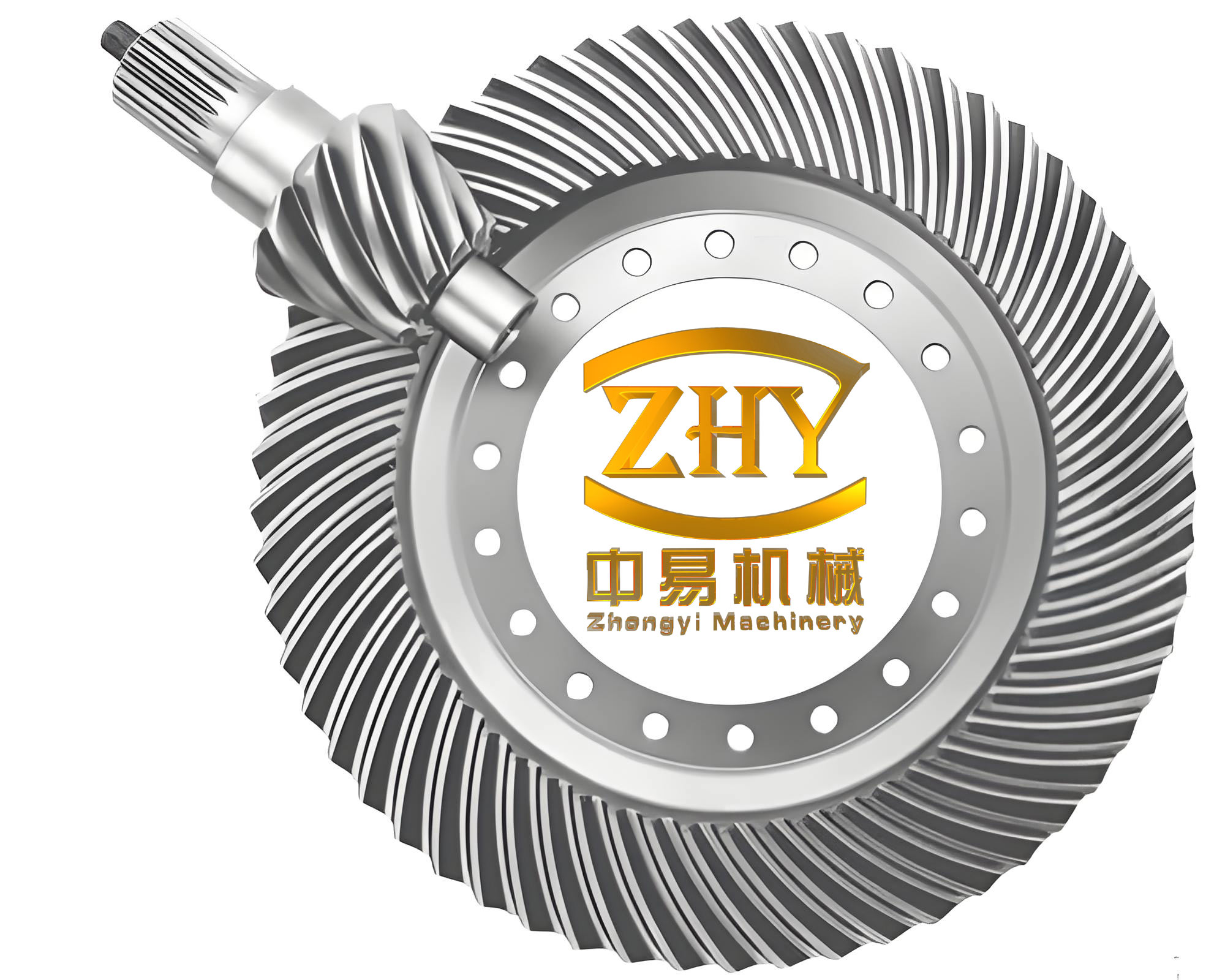
Meshing Geometry and Loaded Contact Analysis of Hypoid Bevel Gears
I first described the spatial meshing relation of the hypoid bevel gears. The pinion axis and gear axis are perpendicular but offset. The pitch point lies on the common tangent plane, and the pitch cones touch along a line that is not parallel to either axis. This offset produces a sliding velocity that changes along the tooth trace and along the tooth profile. For the rear axle hypoid bevel gears considered here, the main geometry is summarized in Table 1.
| Parameter | Pinion | Gear |
|---|---|---|
| Number of teeth | 10 | 43 |
| Mean pressure angle | 19° | 19° |
| Pitch diameter | 63 mm | 180 mm |
| Mean spiral angle | 46°48′ | 28°37′ |
| Pitch cone angle | 18°15′ | 70°42′ |
| Hand of spiral | Left | Right |
| Offset | 25 mm | |
| Shaft angle | 90° | |
| Face width | 34 mm | |
I defined the surface velocity of the pinion and gear at a contact point \(M_{ij}\) by the cross product of angular velocity and position vector. In equation form,
$$ \mathbf{v}_{ij}^{p}=\boldsymbol{\omega}_{p}\times \mathbf{r}_{ij}^{p}, \qquad \mathbf{v}_{ij}^{g}=\boldsymbol{\omega}_{g}\times \mathbf{r}_{ij}^{g} $$
where the superscripts p and g denote the pinion and gear, respectively. The gear ratio relation is
$$ \omega_{p}=R\,\omega_{g} $$
with R being the transmission ratio. I projected the surface velocity onto the common normal and the tangent plane. The normal components are equal for ideal conjugate motion, while the tangential components produce sliding. If the tangent plane is spanned by two orthogonal directions t and t′, then the sliding velocity components are
$$ v_{ij,t}^{s}=(u_{ij}^{p})_{t}-(u_{ij}^{g})_{t} $$
$$ v_{ij,t’}^{s}=(u_{ij}^{p})_{t’}-(u_{ij}^{g})_{t’} $$
The magnitude of the sliding velocity is therefore
$$ v_{ij}^{s}=\sqrt{\left[(v_{ij,t}^{s})\right]^{2}+\left[(v_{ij,t’}^{s})\right]^{2}} $$
Using the actual hypoid bevel gear parameters and a pinion speed of 2000 r/min, I solved the meshing kinematics with a numerical code. I found that the relative sliding speed along the active contact path ranged from about 2 m/s to 8 m/s. The sliding speed increased from the tooth root toward the tooth tip. This range became the input condition for the lubrication simulations.
To obtain the contact location and contact stress, I built a five-tooth finite element model. I simplified the pinion and gear by removing small chamfers, fillets, and threaded holes that do not influence the contact solution. I divided each tooth into several topological blocks so that a mapped hexahedral mesh could be generated. The final model contained 138,071 nodes and 121,372 elements. The material properties assigned to the hypoid bevel gears are listed in Table 2.
| Property | Value |
|---|---|
| Material | 20CrMnTi |
| Elastic modulus | 207 GPa |
| Poisson ratio | 0.25 |
| Density | 7800 kg/m³ |
I set the pinion concave surface as the target surface and the gear convex surface as the contact surface. I used an asymmetric contact pair with a friction coefficient of 0.08. The augmented Lagrange algorithm was selected because it gives a stable contact pressure. To simulate normal driving, I applied a pinion speed ramp and a resisting torque on the gear. The gear load torque was calculated from vehicle weight, rolling radius, road resistance, grade resistance, final drive ratio, and transmission efficiency. The resulting load was 250 N·m. The drive speed and torque were applied through step functions to avoid instantaneous shock.
I validated the finite element contact model by a tooth-contact imprint test. I coated the gear convex surfaces with a mixture of red lead and oil, mounted the final drive on a test fixture, and rotated the hypoid bevel gears at 2000 r/min. After several revolutions, I observed a clear elliptical contact imprint on the gear convex surface. The imprint was located along the tooth length and tooth height in a region consistent with the finite element prediction. The simulation showed that multiple tooth pairs participate in meshing at the same time, which confirms the high contact ratio of the hypoid bevel gears. The maximum equivalent contact stress was about 1364.2 MPa, and the stress peaks appeared periodically with the tooth meshing cycle. These results gave me the contact zone and load level needed for the micro-dimple design.
Two-Dimensional Lubrication Model with Micro-Dimples
After obtaining the contact parameters, I simplified the local contact between one pinion tooth and one gear tooth into a two-dimensional sliding lubrication problem. This simplification is reasonable because the micro-dimple size is much smaller than the tooth surface curvature. I considered three main mechanisms by which surface texture can improve hydrodynamic lubrication: cavitation, inertia, and wedge action. The wedge action arises because the flow gap increases at the dimple inlet and decreases at the dimple outlet. The inlet forms a divergent wedge and the outlet forms a convergent wedge. If the pressure drop and pressure rise do not cancel completely, a net load-carrying capacity is generated.
I used the Navier–Stokes equations as the governing equations for the lubricant. For a Newtonian fluid, the momentum equation is
$$ \rho \frac{Du_i}{Dt}=-\frac{\partial p}{\partial x_i}+\rho G_i+\frac{\partial}{\partial x_j}\left[2\eta\left(e_{ij}-\frac{1}{3}\delta_{ij}\nabla\cdot \mathbf{u}\right)\right] $$
and the continuity equation is
$$ \frac{\partial \rho}{\partial t}+\frac{\partial(\rho u_i)}{\partial x_i}=0 $$
where \(\rho\) is density, \(u_i\) is velocity, \(p\) is pressure, \(\eta\) is dynamic viscosity, and \(e_{ij}\) is the strain-rate tensor. For the thin lubricant film, I assumed an incompressible Newtonian lubricant, constant temperature, constant viscosity, and steady laminar flow. The Reynolds number was defined as
$$ Re=\frac{Lu}{\mu} $$
where L is a characteristic length, u is a characteristic velocity, and \(\mu\) is kinematic viscosity. For the present micro-dimple scale, the Reynolds number is small, so the laminar assumption is appropriate.
I selected four micro-dimple shapes: square, triangular, spherical segment, and trapezoidal. I denoted them by R, T, S, and L, respectively. The dimple width was w, the maximum depth was hmax, the film thickness was h0, and the spacing length was L. The geometric parameters are summarized in Table 3. To relate the dimple depth to the boundary layer thickness, I used the turbulent boundary layer formula
$$ \delta=\frac{0.035x}{Re_x^{1/7}} $$
For a sliding speed of 5 m/s, a spacing of 200 µm, and a lubricant kinematic viscosity of \(5\times10^{-5}\) m²/s, the local Reynolds number was 66.7 and the boundary layer thickness was about 3.84 µm. Therefore, I designed the dimple depths to be of the same order as the boundary layer thickness. The depth values were 1.5, 2.5, 3.5, 4.5, 5.0, 6.5, and 7.5 µm. The width values were 40, 70, 100, 130, 160, and 180 µm. This gave a total of 168 simulation cases for the two-dimensional parametric study.
| Shape | Width values (µm) | Depth values (µm) | Spacing (µm) | Sliding speed (m/s) | Number of cases |
|---|---|---|---|---|---|
| Square (R) | 40, 70, 100, 130, 160, 180 | 1.5, 2.5, 3.5, 4.5, 5, 6.5, 7.5 | 200 | 5 | 168 |
| Triangular (T) | 40, 70, 100, 130, 160, 180 | 1.5, 2.5, 3.5, 4.5, 5, 6.5, 7.5 | 200 | 5 | 168 |
| Spherical segment (S) | 40, 70, 100, 130, 160, 180 | 1.5, 2.5, 3.5, 4.5, 5, 6.5, 7.5 | 200 | 5 | 168 |
| Trapezoidal (L) | 40, 70, 100, 130, 160, 180 | 1.5, 2.5, 3.5, 4.5, 5, 6.5, 7.5 | 200 | 5 | 168 |
To compare results across different sizes, I introduced dimensionless variables:
$$ X=\frac{x}{L}, \quad Y=\frac{y}{h_0}, \quad U=\frac{u}{u_0}, \quad V=\frac{v}{u_0}, \quad P=\frac{p}{p_0} $$
where \(p_0=\eta u_0/L\). The dimensionless Navier–Stokes equations in the x and y directions become
$$ \frac{U\partial U}{\partial X}+\frac{V\partial U}{\partial Y}=-\frac{\partial P}{\partial X}+\frac{1}{Re}\left(\frac{\partial^2 U}{\partial X^2}+\frac{\partial^2 U}{\partial Y^2}\right) $$
$$ \frac{U\partial V}{\partial X}+\frac{V\partial V}{\partial Y}=-\frac{\partial P}{\partial Y}+\frac{1}{Re}\left(\frac{\partial^2 V}{\partial X^2}+\frac{\partial^2 V}{\partial Y^2}\right) $$
and the dimensionless continuity equation is
$$ \frac{\partial U}{\partial X}+\frac{\partial V}{\partial Y}=0 $$
I solved these equations using a commercial CFD solver. The upper wall moved with a specified velocity, the lower wall was fixed, and the left and right boundaries were set as periodic boundaries to represent a continuous dimple array. I refined the mesh near the walls to capture the boundary layer. The pressure–velocity coupling used the SIMPLE algorithm, the pressure term used a second-order scheme, and the momentum term used a QUICK scheme. The convergence criteria for continuity and velocity components were set to \(10^{-15}\).
To evaluate lubrication performance, I defined the following integral quantities:
$$ F_y=\int p\,dx $$
$$ F_x=\int \tau\,dx $$
$$ f=\frac{F_x}{F_y} $$
where \(F_y\) is the oil-film load capacity, \(F_x\) is the wall friction force, \(\tau\) is the wall shear stress, and f is a composite friction coefficient. A larger \(F_y\) and a smaller \(F_x\) indicate better lubrication. In the parametric study, I found that the smooth surface produced almost no net pressure. In contrast, every micro-dimple produced a negative pressure region near the inlet and a positive pressure region near the outlet. The square and trapezoidal dimples produced the largest pressure difference. The triangular dimple produced the smallest pressure difference, and the spherical segment dimple produced an intermediate value.
From the pressure maps and streamlines, I observed that square and trapezoidal dimples formed strong vortex zones at the inlet and outlet. The square dimple produced larger symmetric triangular vortices, while the trapezoidal dimple produced more compact vortices because its sloped walls guide the lubricant. The triangular dimple formed a large vortex at its sharp bottom corner, which weakened the wedge action. The spherical segment dimple formed an elongated elliptical vortex. These flow patterns explain why the square and trapezoidal dimples had better dynamic pressure performance.
For each shape, I identified the optimum width and depth by maximizing the load capacity and minimizing the friction force. The optimal two-dimensional parameters are listed in Table 4.
| Shape | Optimal dimensionless width W | Optimal dimensionless depth H | Maximum positive pressure (dimensionless) | Load capacity rank | Composite coefficient rank |
|---|---|---|---|---|---|
| Square (R) | 0.8 | 0.9 | 0.3225 | 2 | 2 |
| Trapezoidal (L) | 0.8 | 0.9 | 0.3228 | 1 | 1 |
| Spherical segment (S) | 0.8 | 1.3 | 0.2930 | 3 | 3 |
| Triangular (T) | 0.8 | 1.5 | 0.2758 | 4 | 4 |
In terms of load capacity, the trapezoidal and square dimples were nearly identical; the difference was only about 1.06%. In terms of wall friction, the square dimple had the lowest value. The composite coefficient ranking was trapezoidal > square > spherical segment > triangular > smooth. Because the square and trapezoidal dimples had similar two-dimensional performance, I selected them for a further cavitation study.
Cavitation Effect and Sliding Speed Influence
Cavitation occurs when the local pressure falls below the saturation vapor pressure. In a micro-dimple, the inlet divergent wedge easily produces a low-pressure region. If the pressure is low enough, vapor bubbles form, grow, and collapse. In lubrication, cavitation can be beneficial because it breaks the antisymmetry of the pressure field and produces a net load capacity. I therefore introduced a mixture multiphase model and the Schnerr–Sauer cavitation model. The saturation pressure was set to 5000 Pa, and the bubble density constant was \(10^{13}\). I used the coupled algorithm for pressure–velocity coupling and PRESTO! for pressure discretization.
I tested six sliding speeds: 1, 3, 5, 7, 9, and 12 m/s. The results showed that at 1 m/s and 3 m/s the vapor volume fraction was almost zero. At 5 m/s and above, cavitation appeared at the dimple inlet. The cavitation region expanded with increasing speed. Therefore, I concluded that the critical sliding speed for cavitation lies between 3 and 5 m/s. Since the actual sliding speed of the hypoid bevel gears ranges from 2 to 8 m/s, cavitation is likely to occur under normal operating conditions.
I compared the square and trapezoidal dimples at W = 0.8 and H = 0.9 under cavitation. Table 5 summarizes the lubrication performance at a sliding speed of 5 m/s.
| Case | Oil-film load capacity | Wall friction force | Composite coefficient | Increase in load capacity due to cavitation | Reduction in friction due to cavitation |
|---|---|---|---|---|---|
| Square, no cavitation | Reference | Reference | Reference | — | — |
| Square, with cavitation | 1.610 × reference | 0.9954 × reference | 1.616 × reference | 61.0% | 0.46% |
| Trapezoidal, no cavitation | Reference | Reference | Reference | — | — |
| Trapezoidal, with cavitation | 1.394 × reference | 0.9978 × reference | 1.398 × reference | 39.4% | 0.22% |
The square dimple had a larger cavitation region and a more disturbed velocity field than the trapezoidal dimple. The load capacity of the square dimple was 14.2% higher than that of the trapezoidal dimple, and its composite coefficient was 14.5% higher. The wall friction of the square dimple was 0.25% lower. Therefore, considering cavitation, I selected the square micro-dimple with W = 0.8 and H = 0.9 as the optimized two-dimensional shape. In dimensional terms, this corresponds to a width of 160 µm and a depth of 4.5 µm.
Three-Dimensional Micro-Dimple Array Layout
I extended the study to three dimensions. First, I compared a single cylindrical micro-dimple and a single cuboid micro-dimple. Both had the same projected width and depth: 160 µm and 4.5 µm, respectively. The cuboid dimple had a square planform, while the cylindrical dimple had a circular planform. The three-dimensional Navier–Stokes equations were solved with the same assumptions as the two-dimensional case. The load capacity and friction force were defined as
$$ F_y’=\iint p\,ds $$
$$ F_x’=\iint \tau\,ds $$
$$ f’=\frac{F_x’}{F_y’} $$
The comparison is given in Table 6. The cuboid dimple produced a much larger load capacity and a larger composite coefficient. Its wall friction was also lower. I therefore selected the cuboid micro-dimple for the array study.
| Micro-dimple type | Maximum pressure difference | Oil-film load capacity | Wall friction force | Composite coefficient |
|---|---|---|---|---|
| Cylindrical | About 770 Pa | Reference | Reference | Reference |
| Cuboid | About 3769 Pa | 2.686 × reference | 0.942 × reference | 2.844 × reference |
I then built a simplified three-dimensional computational domain representing the meshing gap between one pinion tooth and one gear tooth. I used the contact imprint region as the design area. Because the full contact region is large, I divided the gap into three sections along the tooth length and used the middle section for the micro-dimple array. I designed a \(4\times4\) dimple array to study spacing and arrangement. The transverse spacing was fixed at 200 µm. The longitudinal spacing values were 200, 225, 250, and 275 µm. Two arrangements were considered: square arrangement and staggered arrangement. The sliding speeds were 1, 3, 5, 7, 9, and 12 m/s. This gave 48 cases, as listed in Table 7.
| Arrangement | Transverse spacing (µm) | Longitudinal spacing (µm) | Sliding speed (m/s) | Number of cases |
|---|---|---|---|---|
| Square | 200 | 200, 225, 250, 275 | 1, 3, 5, 7, 9, 12 | 24 |
| Staggered | 200 | 200, 225, 250, 275 | 1, 3, 5, 7, 9, 12 | 24 |
The three-dimensional CFD model used a mixture of tetrahedral and prismatic elements. Boundary layers were placed on the upper wall and on the dimple surfaces. The first layer height was 0.12 µm, the growth rate was 1.2, and the non-boundary-layer mesh size was limited to 3 µm. The mesh size was about 540,000 elements for a single dimple. The same solver settings as in the two-dimensional case were used.
The pressure distribution showed that in the square arrangement, the pressure curves along three lines parallel to the sliding direction were periodic. The amplitude decreased from the center line toward the side lines, which means that neighboring dimples in the same row interact weakly. The longitudinal spacing controls the continuity of pressure between adjacent rows. In the staggered arrangement, the pressure curves were also periodic, but the period became shorter because the high-pressure region of one row was adjacent to the low-pressure region of the next row. The transverse pressure curve showed that the longitudinal spacing is the key parameter for the overall dynamic pressure effect.
The average dimensionless pressure and load capacity results are summarized in Table 8. For the square arrangement, the load capacity was positive and decreased as longitudinal spacing increased. For the staggered arrangement, the load capacity was negative under all conditions. This means that the staggered arrangement did not produce a net load-carrying film in the present geometry. The square arrangement with a longitudinal spacing of 200 µm gave the highest load capacity.
| Arrangement | Longitudinal spacing (µm) | Average dimensionless pressure | Load capacity | Wall friction force | Composite coefficient |
|---|---|---|---|---|---|
| Square | 200 | Highest positive | Highest positive | Lowest | Best |
| Square | 225 | Lower | Lower | Slightly higher | Lower |
| Square | 250 | Much lower | Much lower | Higher | Lower |
| Square | 275 | Lowest positive | Lowest positive | Highest | Worst among square |
| Staggered | 200 | Negative | Negative | Comparable | Negative |
| Staggered | 275 | Least negative | Least negative | Comparable | Least negative |
From the three-dimensional array study, I concluded that the cuboid micro-dimple with length 160 µm, width 160 µm, and depth 4.5 µm, arranged in a square pattern with both transverse and longitudinal spacing of 200 µm, gives the best lubrication performance for the hypoid bevel gears. This array design was then transferred to the tooth surface for dynamic analysis.
Dynamic Simulation of Hypoid Bevel Gears with Micro-Dimple Tooth Surfaces
I built two virtual prototypes: one with smooth tooth surfaces and one with micro-dimple arrays on selected gear convex surfaces. The micro-dimple array was created in a CAD environment. On each selected gear tooth, I placed 20 dimples along the tooth height and 80 dimples along the tooth length, giving 1600 dimples per tooth surface. Then I exported the models to ADAMS. The micro-dimple array was oriented along the tooth length so that the dimple rows would not coincide with the meshing line. This preserves the original meshing condition of the hypoid bevel gears.
The meshing condition for the hypoid bevel gears can be written as
$$ \mathbf{n}\cdot \mathbf{v}=0 $$
where n is the normal vector at a contact point and v is the relative velocity between the pinion and gear. Because the micro-dimple depth is only a few micrometers, it does not change the macroscopic curvature of the tooth surface. Therefore, the original meshing condition is essentially maintained.
In ADAMS, I defined the material properties, revolute joints, contact forces, friction, drive speed, and load torque. The contact stiffness was calculated from
$$ K=\frac{4}{3}R^{1/2}E^{*} $$
where
$$ \frac{1}{R}=\frac{1}{R_1}+\frac{1}{R_2} $$
$$ \frac{1}{E^{*}}=\frac{1-\mu_1^2}{E_1}+\frac{1-\mu_2^2}{E_2} $$
Using the equivalent radii and the material properties of the hypoid bevel gears, the contact stiffness was \(6.565\times10^5\) N/mm. The force exponent was 1.5, the penetration depth was 0.1 mm, and the damping coefficient was 100 N·s/mm. The static friction coefficient was 0.08, the dynamic friction coefficient was 0.05, the static transition velocity was 0.1 mm/s, and the dynamic transition velocity was 10 mm/s. The contact parameter settings are summarized in Table 9.
| ADAMS contact parameter | Value |
|---|---|
| Contact stiffness | \(6.565\times10^5\) N/mm |
| Force exponent | 1.5 |
| Penetration depth | 0.1 mm |
| Damping coefficient | 100 N·s/mm |
| Static friction coefficient | 0.08 |
| Dynamic friction coefficient | 0.05 |
| Static transition velocity | 0.1 mm/s |
| Dynamic transition velocity | 10 mm/s |
The drive speed and load torque were applied with step functions. The pinion speed increased from zero to 2000 r/min within 0.2 s, and the gear load increased from zero to 250 N·m within 0.2 s. The simulation time was 0.8 s with a time step of \(10^{-4}\) s. I first validated the smooth model. The theoretical gear speed was 2790.70 deg/s. The simulated average gear speed was 2790.6975 deg/s, which is very close to the theoretical value. The load torque also followed the prescribed step function. This confirmed that the virtual prototype was correct.
I then compared the smooth and micro-dimpled hypoid bevel gears. The transmission error was defined as
$$ TE=\frac{\left|\omega_{g,\text{theory}}-\omega_{g,\text{sim}}\right|}{\omega_{g,\text{theory}}}\times 100\% $$
For the smooth hypoid bevel gears, the transmission error was 0.0014%. For the micro-dimpled hypoid bevel gears, the transmission error was 0.0022%. The difference was only 0.0008%, which indicates that the micro-dimple array has almost no effect on the transmission error. The gear angular velocity showed small periodic fluctuations when the micro-dimpled teeth were in mesh, but the overall transmission stability was maintained.
The meshing force results are given in Table 10. The average meshing force of the smooth pair was 3188.0196 N. The average meshing force of the micro-dimpled pair was 3208.5083 N. The increase was 20.4887 N, or 0.64%. This small increase is acceptable for the lubrication benefit obtained.
| Quantity | Smooth hypoid bevel gears | Micro-dimpled hypoid bevel gears | Difference |
|---|---|---|---|
| Transmission error | 0.0014% | 0.0022% | 0.0008% |
| Average meshing force | 3188.0196 N | 3208.5083 N | 20.4887 N (0.64%) |
| Maximum force peak in frequency domain | 133.12 N | 122.43 N | 10.69 N reduction |
| Dominant frequency components | 333, 666, 1000, 1333, 1666, 2000 Hz | 333, 666, 1000, 1333, 1666, 2000 Hz | Essentially the same |
I also examined the frequency content of the meshing force. The fundamental meshing frequency of the hypoid bevel gears was 333 Hz, with harmonics at 666, 1000, 1333, 1666, and 2000 Hz. The smooth pair and the micro-dimpled pair had nearly the same frequency components. However, the micro-dimpled pair showed a slightly more complex frequency spectrum, with small side peaks near the main peaks. The maximum force peak in the frequency domain decreased from 133.12 N to 122.43 N. This suggests that the micro-dimple array may slightly reduce the peak dynamic excitation while maintaining the overall meshing characteristics.
Overall Findings and Engineering Implications
My study shows that micro-dimples can be used to improve the lubrication of hypoid bevel gears without seriously degrading their meshing dynamics. The main findings are as follows. First, the relative sliding speed of the hypoid bevel gears ranges from 2 to 8 m/s, and the contact imprint is located on the gear convex surface in a well-defined elliptical region. Second, the square micro-dimple with a width of 160 µm and a depth of 4.5 µm gives the best two-dimensional lubrication performance when cavitation is considered. Third, a cuboid micro-dimple with length and width of 160 µm and depth of 4.5 µm, arranged in a square array with 200 µm spacing, gives the best three-dimensional lubrication performance. Fourth, the micro-dimple array increases the average meshing force by only 0.64% and changes the transmission error by only 0.0008%. These results support the use of micro-dimple tooth surfaces in hypoid bevel gears for friction reduction and vibration control.
From an engineering perspective, the design procedure I followed can be summarized as a sequence of steps. I first obtained the contact zone and sliding speed. I then used a two-dimensional CFD model to screen micro-dimple shapes and sizes. I next used a three-dimensional CFD model to optimize the array spacing and arrangement. Finally, I used a dynamic simulation to verify that the texture does not harm the meshing behavior. This sequence is practical because it reduces the number of expensive full-scale experiments and provides a rational basis for choosing texture parameters.
The main limitation of my work is that I assumed constant lubricant temperature and viscosity. In real hypoid bevel gears, friction heating changes viscosity and film thickness, so a thermal elastohydrodynamic model would be more accurate. Another limitation is that the three-dimensional array model used a simplified flat contact domain rather than the actual curved tooth surface. Future work should include thermal effects, transient effects, and real tooth-surface curvature. Nevertheless, the present results provide a useful foundation for the design of micro-dimpled hypoid bevel gears and for further studies on their lubrication and dynamics.