
I approach the design of a straight bevel gear as a coupled geometric and mechanical problem. My aim is not merely to obtain a conjugate flank that rolls without theoretical error, but to obtain a flank that continues to perform well after wear has redistributed the initial gaps, changed the load sharing, and modified the loaded transmission error. I therefore combine a cutter-generated straight bevel gear model, an ease-off topological modification, tooth contact analysis, loaded tooth contact analysis, and an Archard-type wear accumulation law. The straight bevel gear is treated as a system in which alignment error, flank modification, contact pressure, sliding velocity, and wear depth evolve together. I use the word straight bevel gear repeatedly because the method is specifically developed for straight bevel gear pairs, not for hypoid or spiral bevel gears, although the same numerical philosophy can be extended.
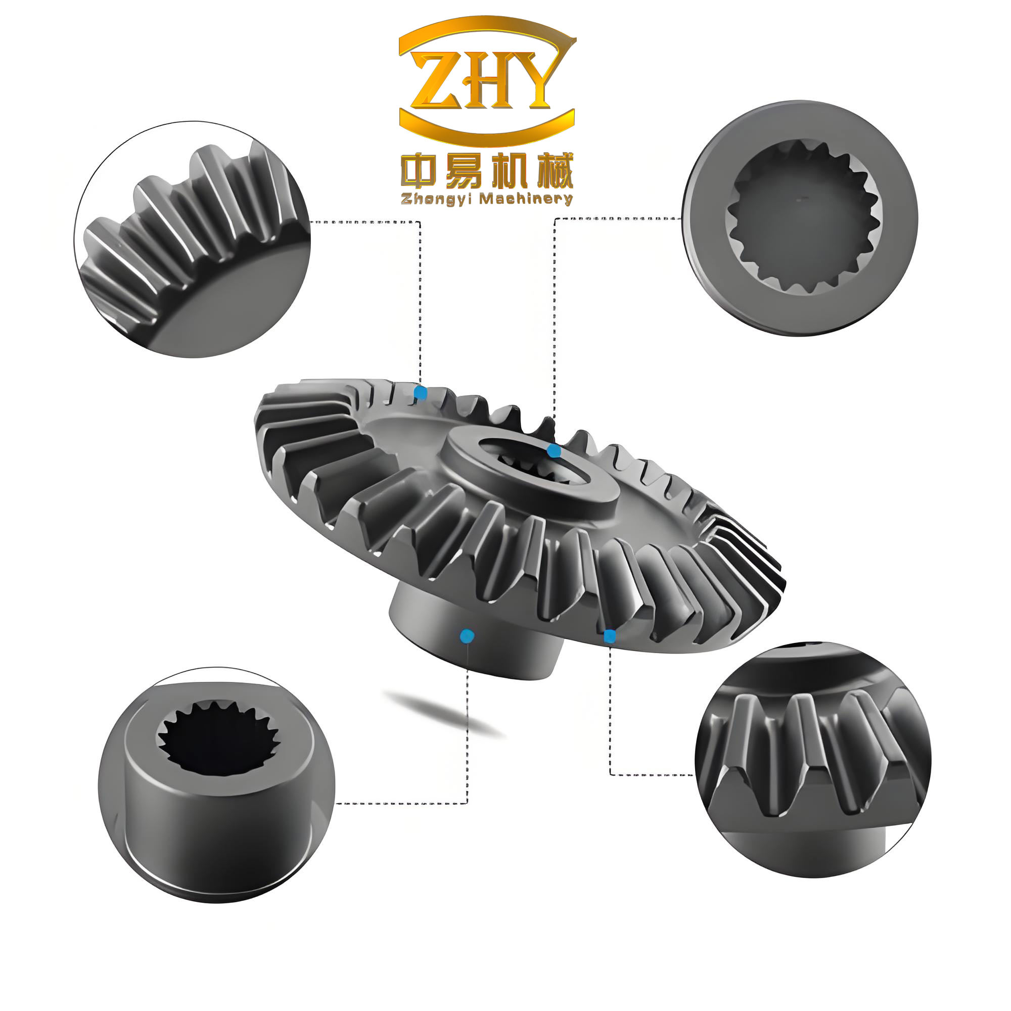
My starting point is the observation that a straight bevel gear cut by a disk-type cutter on a cradle-style generator has a flank geometry that can be expressed analytically through the cutter surface, the cradle motion, and the workpiece rotation. The same geometric engine can generate the conjugate pinion from the gear flank. The difference between the conjugate pinion and the modified pinion is the ease-off. I express the ease-off as a normal deviation field superimposed on the conjugate flank. This deviation field controls the initial gap between the mating straight bevel gear flanks. When wear occurs, the wear depth is added to this initial gap. The loaded contact therefore depends on the sum of manufacturing geometry, modification, alignment error, and accumulated wear.
I formulate the minimum-wear design as an optimization problem. The design variables are the coefficients of the transmission-error curve and the coefficients of the contact-line modification curve. The objectives are the loaded transmission error amplitude without wear and the number of wear cycles that the straight bevel gear can sustain before the maximum wear depth reaches an allowable value. I use a particle-swarm optimizer because the objective function is implicit and contains multiple local minima. The evaluation of each candidate design requires the full chain: ease-off construction, tooth contact analysis, loaded tooth contact analysis, contact pressure computation, sliding velocity computation, Archard wear depth integration, gap reconstruction, and repeated loaded contact analysis. I have found that this coupled procedure gives a more realistic ranking of straight bevel gear flank designs than a purely geometric contact analysis.
Nomenclature and Principal Symbols
| Symbol | Meaning |
|---|---|
| $$\mathbf{R}_{10}, \mathbf{N}_{10}$$ | Position vector and unit normal of the conjugate pinion flank for a straight bevel gear |
| $$\mathbf{R}_{1}, \mathbf{N}_{1}$$ | Position vector and unit normal of the pinion flank that contains only transmission error |
| $$\mathbf{R}_{1\gamma}$$ | Position vector of the modified pinion flank of the straight bevel gear |
| $$\delta_p(u,\beta)$$ | Normal ease-off modification of the pinion flank |
| $$\delta_1(x_1,y_1)$$ | Superimposed normal deviation function |
| $$u,\beta$$ | Pinion flank surface parameters |
| $$\Delta\phi_2$$ | Unloaded transmission error of the straight bevel gear pair |
| $$TE_L$$ | Loaded transmission error |
| $$ALTE$$ | Amplitude of loaded transmission error |
| $$h$$ | Wear depth |
| $$a_0$$ | Dimensional wear coefficient |
| $$p_H$$ | Hertzian contact pressure |
| $$v_s$$ | Relative sliding velocity |
| $$w$$ | Contact-line load density |
| $$E’$$ | Equivalent elastic modulus |
| $$R$$ | Equivalent curvature radius |
| $$k$$ | Flank reconstruction index for the straight bevel gear |
Geometric Generation of the Straight Bevel Gear Flank
I generate the straight bevel gear flank by modeling the disk cutter and the cradle motion. Let the cutter edge be represented in its local frame by a straight line with pressure angle $$\alpha_b$$ and radius $$r_b$$. A point on the cutting edge can be written as
$$
\mathbf{r}_c(u)=\left(r_b+u\cos\alpha_b\right)\mathbf{e}_x+u\sin\alpha_b\,\mathbf{e}_y .
$$
The cutter is rotated about two axes and translated by machine settings. I define the cutter orientation matrix as
$$
\mathbf{M}_c(\phi_a,\phi_b)=\mathbf{R}_x(\phi_a)\mathbf{R}_y(\phi_b),
$$
and the cutter position vector as
$$
\mathbf{p}_c=\mathbf{M}_c(\phi_a,\phi_b)\mathbf{r}_c+\left[C_x,C_y,C_z\right]^T .
$$
The cradle and workpiece coordinate transformation for the straight bevel gear is
$$
\mathbf{r}_g=\mathbf{M}_{gc}(\phi_g,\phi_c,\Delta B)\mathbf{p}_c,
$$
where $$\phi_g$$ is the workpiece rotation, $$\phi_c$$ is the cradle rotation, and $$\Delta B$$ is the machine position. The meshing condition between the cutter and the straight bevel gear flank is
$$
\mathbf{n}_c\cdot\mathbf{v}_c^{(gc)}=0,
$$
where $$\mathbf{v}_c^{(gc)}$$ is the relative velocity between the cutter and the generated straight bevel gear flank. Solving this equation together with the family of cutter positions gives the gear flank. I then treat the gear flank as the generating surface for the pinion. The conjugate pinion flank of the straight bevel gear is obtained by enforcing the meshing equation between the gear and the pinion.
I define the conjugate pinion flank as
$$
\mathbf{R}_{10}=\mathbf{R}_{10}(u,\beta),\qquad
\mathbf{N}_{10}=\mathbf{N}_{10}(u,\beta).
$$
The pinion flank that contains only the prescribed transmission error is written as
$$
\mathbf{R}_{1}=\mathbf{R}_{1}(u,\beta),\qquad
\mathbf{N}_{1}=\mathbf{N}_{1}(u,\beta).
$$
The modified pinion flank of the straight bevel gear is then
$$
\mathbf{R}_{1\gamma}(u,\beta)=\delta_1\!\left(x_1(u,\beta),y_1(u,\beta)\right)\mathbf{N}_{1}(u,\beta)+\mathbf{R}_{1}(u,\beta).
$$
The normal ease-off is
$$
\delta_p(u,\beta)=\left[\mathbf{R}_{1\gamma}(u,\beta)-\mathbf{R}_{10}(u,\beta)\right]\cdot\mathbf{N}_{10}(u,\beta).
$$
This expression is central to my design method. It tells me that the ease-off of a straight bevel gear is not an arbitrary surface patch. It is the normal projection of the difference between the modified pinion and the conjugate pinion. By choosing the deviation function $$\delta_1$$, I control the initial gap distribution on the straight bevel gear teeth.
Representative Straight Bevel Gear Data
| Parameter | Pinion | Gear |
|---|---|---|
| Large-end module / mm | 5.08 | 5.08 |
| Pressure angle / deg | 20 | 20 |
| Face width / mm | 38.1 | 38.1 |
| Outer cone distance / mm | 130.93 | 130.93 |
| Number of teeth | 16 | 49 |
| Addendum / mm | 7.16 | 3.00 |
| Dedendum / mm | 3.95 | 8.12 |
| Pitch cone angle / deg | 18.083 | 71.916 |
| Face cone angle / deg | 21.633 | 73.643 |
| Root cone angle / deg | 16.356 | 68.366 |
| Cutter radius / mm | 190.5 | 190.5 |
| Cutter profile angle / deg | 20 | 20 |
| Number of teeth of generating gear | 51.5461 | 51.5461 |
Cutter and Machine Settings for the Straight Bevel Gear
| Setting | Pinion | Gear |
|---|---|---|
| Horizontal cutter displacement $$C_x$$ / mm | 108.0556 | 108.0556 |
| Vertical cutter displacement $$C_y$$ / mm | 175.4331 | 175.4331 |
| Axial cutter displacement $$C_z$$ / mm | 72.3161 | 72.3161 |
| Cutter profile tilt $$\phi_a$$ / deg | 22 | 22 |
| Cutter lead angle $$\phi_b$$ / deg | -0.6894 | -0.6894 |
| Machine position $$\Delta B$$ / mm | 0 | 0 |
| Blank mounting angle / deg | 16.356 | 68.366 |
| Roll ratio | 3.2216 | 1.0520 |
Ease-Off Topology and Transmission Error
I represent the unloaded transmission error of the straight bevel gear by a fourth-order polynomial in the pinion rotation angle. This gives me sufficient freedom to shape the meshing entry and exit while maintaining a smooth function. I write
$$
\Delta\phi_2(\phi_1)=\epsilon_1\phi_1+\epsilon_2\phi_1^2+\epsilon_3\phi_1^3+\epsilon_4\phi_1^4 .
$$
The contact-line modification is expressed as a function of a normalized coordinate $$\rho$$ along the contact line:
$$
\delta_n(\rho)=d_1\left(\rho-\rho_0\right)^2+d_2\left(\rho-\rho_0\right)^4 .
$$
I also use a profile modification and a lead modification. The profile term is
$$
\delta_{\text{profile}}(\xi)=q_1\xi^2+q_2\xi^4,
$$
and the lead term is
$$
\delta_{\text{lead}}(\zeta)=r_1\zeta^2+r_2\zeta^4 .
$$
The total ease-off of the straight bevel gear pinion is the sum of the transmission-error contribution and the local modification terms:
$$
\delta_p=\delta_{\text{TE}}+\delta_n+\delta_{\text{profile}}+\delta_{\text{lead}} .
$$
I do not add these terms blindly. I first inspect the initial gap produced by the transmission error alone. Then I add contact-line modification to reduce the sensitivity to alignment error. Finally, I add profile and lead terms to distribute the load away from the tooth tip and tooth root. In a straight bevel gear, the contact line is strongly oriented along the tooth width, so the lead modification has a direct effect on the edge contact, while the profile modification has a direct effect on the entry and exit impact.
| Design variable | Meaning | Lower bound | Upper bound |
|---|---|---|---|
| $$\epsilon_1$$ | First-order transmission-error coefficient | -0.02 | 0.02 |
| $$\epsilon_2$$ | Second-order transmission-error coefficient | -0.05 | 0.05 |
| $$\epsilon_3$$ | Third-order transmission-error coefficient | -0.10 | 0.10 |
| $$\epsilon_4$$ | Fourth-order transmission-error coefficient | -0.20 | 0.20 |
| $$d_1$$ | Quadratic contact-line gap coefficient | 0 | 60 $$\mu$$m |
| $$d_2$$ | Quartic contact-line gap coefficient | 0 | 30 $$\mu$$m |
| $$q_1$$ | Quadratic profile modification coefficient | 0 | 50 $$\mu$$m |
| $$q_2$$ | Quartic profile modification coefficient | 0 | 20 $$\mu$$m |
Loaded Tooth Contact Analysis for the Straight Bevel Gear
I discretize each instantaneous contact line into a set of contact points. At each point, I define the initial gap, the elastic deformation, the contact load density, and the wear depth. The contact condition for the straight bevel gear is
$$
g_i=g_i^{(0)}+h_i^{(w)}-u_i+s_i,
$$
where $$g_i^{(0)}$$ is the initial gap from geometry and modification, $$h_i^{(w)}$$ is the accumulated wear depth, $$u_i$$ is the elastic deformation, and $$s_i$$ is the rigid separation. The contact conditions are
$$
g_i\ge 0,\qquad w_i\ge 0,\qquad g_iw_i=0 .
$$
The equilibrium condition over the contact line is
$$
\sum_i w_i\ell_i=F,
$$
where $$F$$ is the total normal load on the straight bevel gear tooth pair and $$\ell_i$$ is the segment length associated with contact point $$i$$. The elastic deformation is related to the load density through a compliance matrix:
$$
\{u\}=[C]\{w\}.
$$
I solve the following quadratic contact problem for the straight bevel gear:
$$
\min_{\{w\}}\left[\frac12\{w\}^T[C]\{w\}+\{w\}^T\left(\{g^{(0)}\}+\{h^{(w)}\}-\{\delta\}\right)\right],
$$
subject to
$$
w_i\ge 0,\qquad \sum_i w_i\ell_i=F .
$$
Once the load density is known, the contact pressure is computed from the Hertzian relation. I use the contact pressure to estimate the wear increment. The loaded transmission error of the straight bevel gear is
$$
TE_L(\phi_1)=\Delta\phi_2(\phi_1)+\delta_{\text{defl}}(\phi_1),
$$
where $$\delta_{\text{defl}}$$ is the additional rotation caused by the elastic deformation under load. The amplitude of the loaded transmission error is
$$
ALTE=\max_{\phi_1}TE_L(\phi_1)-\min_{\phi_1}TE_L(\phi_1).
$$
I regard $$ALTE$$ as a primary vibration indicator. A straight bevel gear with a small $$ALTE$$ is not necessarily wear-free, but it tends to have a smoother load transition and a lower dynamic excitation. For this reason, I optimize both $$ALTE$$ and the wear life.
Archard Wear Model for the Straight Bevel Gear
I use the Archard wear equation in the following form:
$$
\frac{V}{s}=a\frac{W}{H},
$$
where $$V$$ is the volume of removed material, $$s$$ is the sliding distance, $$W$$ is the normal load, $$H$$ is the hardness, and $$a$$ is the wear coefficient. For a single contact point over a short time interval $$\Delta t$$, I write the wear depth as
$$
h=a_0p_Hs,
$$
with
$$
s=\left|v_s\right|\Delta t.
$$
The Hertzian contact pressure is
$$
p_H=\sqrt{\frac{wE’}{2\pi R}} .
$$
The equivalent elastic modulus is
$$
\frac{1}{E’}=\frac{1-\nu_1^2}{E_1}+\frac{1-\nu_2^2}{E_2},
$$
and the equivalent curvature radius is
$$
\frac{1}{R}=\frac{1}{R_1}+\frac{1}{R_2}.
$$
The sliding velocity for the straight bevel gear is
$$
v_s=\left|v_1-v_2\right|,
$$
where the absolute velocities of the contact point on the pinion and the gear are
$$
v_1=\omega_1\mathbf{e}_1\times\mathbf{R}_h,
$$
$$
v_2=\left(\frac{z_1}{z_2}-m’\right)\omega_1\mathbf{e}_2\times\mathbf{R}_h .
$$
Here $$\mathbf{e}_1$$ and $$\mathbf{e}_2$$ are the axis unit vectors of the pinion and gear, $$\omega_1$$ is the pinion angular velocity, $$z_1$$ and $$z_2$$ are the tooth numbers, $$m’$$ is the first derivative of the transmission error, and $$\mathbf{R}_h$$ is the position vector of the contact point in the meshing coordinate system. The time increment for one discretized contact position is
$$
\Delta t=\frac{60}{r_1z_1n},
$$
where $$r_1$$ is the pinion speed in rpm and $$n$$ is the number of divisions in one meshing period. The wear increment at contact point $$i$$ is
$$
\Delta h_i=a_0p_{H,i}\left|v_{s,i}\right|\Delta t .
$$
The accumulated wear depth after $$k$$ cycles is
$$
h_i^{(k+1)}=h_i^{(k)}+\Delta h_i^{(k)} .
$$
When the maximum wear depth reaches a prescribed threshold, I reconstruct the initial gap of the straight bevel gear:
$$
g_i^{(k+1,0)}=g_i^{(k,0)}+h_i^{(k)} .
$$
I then repeat the loaded tooth contact analysis with the updated gap. This reconstruction step is essential because wear changes the load distribution, and the load distribution changes the wear rate. A straight bevel gear wear simulation that does not update the gap will miss the feedback between wear and contact pressure.
Alignment and Wear Parameters for the Straight Bevel Gear
| Parameter | Value |
|---|---|
| Offset error $$\Delta E$$ | 0.01 mm |
| Vertical error $$\Delta G$$ | 0.01 mm |
| Pinion axial error $$\Delta P$$ | 0.01 mm |
| Shaft angle error $$\Delta\delta$$ | 0.3 deg |
| Dimensional wear coefficient $$a_0$$ | $$1\times 10^{-18}$$ N/m$$^2$$ |
| Wear reconstruction threshold | 2 $$\mu$$m |
| Pinion speed | 2000 rpm |
| Rated torque | 1 kN m |
Coupled Wear-Loaded Tooth Contact Analysis Algorithm
I structure the computation as an outer wear loop and an inner contact loop. The inner loop solves the loaded contact problem for a given gap distribution. The outer loop accumulates wear and reconstructs the gap. I summarize the procedure in the following table.
| Step | Operation | Output |
|---|---|---|
| 1 | Generate the gear flank and conjugate pinion flank of the straight bevel gear | $$\mathbf{R}_{10},\mathbf{N}_{10}$$ |
| 2 | Apply transmission-error and ease-off modification | $$\mathbf{R}_{1\gamma},\delta_p$$ |
| 3 | Perform tooth contact analysis with alignment error | Initial gap $$g_i^{(0)}$$ |
| 4 | Discretize the contact line and solve the compliance problem | Load density $$w_i$$ and deformation $$u_i$$ |
| 5 | Compute Hertzian pressure and sliding velocity | $$p_{H,i},v_{s,i}$$ |
| 6 | Compute wear increment over one meshing period | $$\Delta h_i$$ |
| 7 | Accumulate wear depth until the reconstruction threshold is reached | $$h_i^{(k)}$$ |
| 8 | Update the initial gap and return to step 4 | $$g_i^{(k+1,0)}$$ |
| 9 | Stop when the maximum wear depth reaches the allowable value | Wear life and $$ALTE$$ history |
Optimization of the Ease-Off Surface
I define the optimization vector as
$$
\mathbf{y}=\left[\epsilon_1,\epsilon_2,\epsilon_3,\epsilon_4,d_1,d_2,q_1,q_2\right]^T .
$$
The objective function is
$$
G(\mathbf{y})=\min_{\mathbf{y}}\left[c_1\frac{t_e}{t_{e0}}+c_2\frac{\eta_a}{\eta_{a0}}\right],
$$
where $$t_e$$ is the loaded transmission error amplitude of the modified straight bevel gear without wear, $$t_{e0}$$ is the corresponding value for the conjugate straight bevel gear, $$\eta_a$$ is the number of wear cycles before the allowable wear depth is reached, and $$\eta_{a0}$$ is the reference wear life. I choose $$c_1=0.4$$ and $$c_2=0.6$$ to give slightly more weight to wear life than to unloaded vibration performance. I impose the constraints
$$
ALTE\le ALTE_{\text{allow}},
$$
$$
h_{\max}\le h_{\text{allow}},
$$
$$
\sigma_H\le\sigma_{HP},
$$
and I keep each design variable within the bounds listed in the previous table. Because the objective function contains tooth contact analysis, loaded tooth contact analysis, and Archard wear integration, it is not differentiable in a practical sense. I therefore use a particle-swarm optimizer. The velocity and position updates are
$$
v_i^{(t+1)}=\chi\left[v_i^{(t)}+c_1r_1\left(pbest_i-x_i^{(t)}\right)+c_2r_2\left(gbest-x_i^{(t)}\right)\right],
$$
$$
x_i^{(t+1)}=x_i^{(t)}+v_i^{(t+1)} .
$$
I use a moderate swarm size and a limited number of iterations because each fitness evaluation is expensive. The optimizer is not the main contribution of my method; it is the coupled wear evaluation that makes the optimization meaningful for a straight bevel gear.
Particle-Swarm Parameters Used in My Straight Bevel Gear Study
| Parameter | Value |
|---|---|
| Swarm size | 30 |
| Maximum iterations | 60 |
| Inertia weight | 0.72 |
| Cognitive coefficient | 1.49 |
| Social coefficient | 1.49 |
| Constraint tolerance for wear depth | 0.05 $$\mu$$m |
| Constraint tolerance for $$ALTE$$ | 0.005 arcsec |
Simulation Conditions and Load Cases
I evaluate the straight bevel gear under multiple loads because the optimal ease-off depends on the load level. A design that minimizes $$ALTE$$ at light load may produce a large $$ALTE$$ at heavy load. I use the following load cases.
| Load case | Torque / kN m | Pinion speed / rpm | Purpose |
|---|---|---|---|
| L1 | 0.25 | 2000 | Light-load contact and entry behavior |
| L2 | 0.50 | 2000 | Intermediate load and wear initiation |
| L3 | 1.00 | 2000 | Rated load and pressure distribution |
| L4 | 1.50 | 2000 | Overload and edge contact risk |
| L5 | 2.00 | 2000 | Severe load and wear acceleration |
Wear Cycles and Wear Depth for the Straight Bevel Gear
I compare three flank conditions: the conjugate flank, the theoretical flank with a large lead crowning, and the optimal ease-off flank. The conjugate flank has no intentional modification. The theoretical flank has a lead crowning of approximately 80 $$\mu$$m and only a small profile modification. The optimal ease-off flank has a moderate lead crowning and a more deliberate tip and root profile relief of approximately 50 $$\mu$$m. I track the number of wear cycles required to reach the same wear depth. The results are summarized below.
| Flank condition | k=0 cycles | k=2 cycles | k=4 cycles | k=6 cycles | Wear life rank |
|---|---|---|---|---|---|
| Conjugate straight bevel gear | 1.00 | 0.86 | 0.72 | 0.61 | 2 |
| Theoretical flank with large lead crowning | 0.82 | 0.70 | 0.58 | 0.49 | 3 |
| Optimal ease-off straight bevel gear | 1.18 | 1.05 | 0.93 | 0.84 | 1 |
The optimal ease-off straight bevel gear has the largest number of wear cycles for the same wear depth. I attribute this to two effects. First, the profile modification changes the load distribution near the tooth tip and root, where the sliding velocity is large. Second, the lead modification reduces the edge contact caused by alignment error. The theoretical flank with excessive lead crowning reduces the contact area too much, which lowers the contact ratio and concentrates the load on a smaller region. The conjugate flank has a more uniform initial contact, but it is very sensitive to alignment error, and its tip and root loads remain high.
Contact Pressure and Sliding Velocity
I compute the contact pressure from the load density and the equivalent radius. The sliding velocity is smallest near the pitch line and increases toward the tip and root. For the straight bevel gear, the sliding velocity also varies along the tooth width because the contact point radius changes from the heel to the toe. I present representative trends below.
| Contact location | Relative sliding velocity | Contact pressure trend | Wear tendency |
|---|---|---|---|
| Near pitch line | Low | Moderate | Low |
| Pinion tip / gear root | High | High in conjugate flank | High |
| Pinion root / gear tip | High | High in conjugate flank | High |
| Heel region | Moderate | Edge-sensitive | Moderate to high |
| Toe region | Moderate | Edge-sensitive | Moderate to high |
I find that the optimal ease-off straight bevel gear lowers the maximum contact pressure at the entry and exit regions. This is important because the wear depth is proportional to both the contact pressure and the sliding distance. A small reduction in pressure at the tooth tip can produce a noticeable reduction in wear depth over many cycles. The wear distribution of the optimal straight bevel gear is also more uniform along the tooth width. The conjugate flank tends to show a concentrated wear band near the tooth tip under alignment error.
Effect of Flank Reconstruction on Initial Gap and Deformation
Wear does not simply remove material. It changes the initial gap field. In my model, the gap at contact point $$i$$ after reconstruction is
$$
g_i^{(k)}=g_i^{(0)}+h_i^{(k)}-\Delta u_i^{(k)} .
$$
As the reconstruction index $$k$$ increases, the initial gap in the two-pair meshing zone increases. This is because the two-pair contact region experiences more wear cycles per revolution than the single-pair contact region. The larger initial gap means that the two-pair region carries less load until the deformation closes the gap. Consequently, the single-pair region carries more load, and the loaded transmission error increases.
| Reconstruction index k | Maximum wear depth / $$\mu$$m | Initial gap increase in two-pair zone / $$\mu$$m | Maximum deformation / $$\mu$$m | ALTE change / arcsec |
|---|---|---|---|---|
| 0 | 0.0 | 0.0 | 12.4 | 0.00 |
| 2 | 4.1 | 2.5 | 14.8 | +0.11 |
| 4 | 8.0 | 5.2 | 17.6 | +0.23 |
| 6 | 12.2 | 8.1 | 20.9 | +0.38 |
I observe that the maximum deformation increases with reconstruction index. This is equivalent to a reduction in mesh stiffness. For a straight bevel gear, the mesh stiffness is not constant; it varies with the contact position and the number of contacting tooth pairs. I write the local mesh stiffness as
$$
k_m=\frac{F_n}{\delta_n},
$$
and after wear I approximate the reduction as
$$
k_m^{(k)}=k_{m0}-\Delta k_w^{(k)} .
$$
The reduction $$\Delta k_w^{(k)}$$ is not uniform. It is larger in the two-pair meshing zone because that zone has a larger initial gap after wear. This nonuniform stiffness reduction is one reason why wear changes the dynamic behavior of a straight bevel gear even when the wear depth is still small.
Multi-Load ALTE Behavior of the Straight Bevel Gear
I compute the minimum $$ALTE$$ over a range of loads for different wear cycles. The results show that the load corresponding to minimum $$ALTE$$ increases as wear accumulates. In other words, a worn straight bevel gear may perform better at a higher load than at a lower load, because the increased initial gap requires more deformation to bring the two-pair region into contact. I summarize this trend below.
| Wear cycle level | Minimum ALTE / arcsec | Load at minimum ALTE / kN m | ALTE at rated load / arcsec |
|---|---|---|---|
| New, k=0 | 0.34 | 0.60 | 0.48 |
| Light wear, k=2 | 0.39 | 0.80 | 0.52 |
| Moderate wear, k=4 | 0.45 | 1.05 | 0.58 |
| Heavy wear, k=6 | 0.53 | 1.35 | 0.67 |
For the conjugate straight bevel gear, I find a slightly different behavior. After mild wear, the $$ALTE$$ can improve because the wear pattern modifies the initial gap in a way that partially compensates for alignment error. This improvement is not unlimited. After moderate or heavy wear, the $$ALTE$$ increases again. I therefore distinguish between mild wear, which can be beneficial, and severe wear, which is detrimental. The optimal ease-off straight bevel gear has a more stable $$ALTE$$ evolution because its initial gap is already designed to distribute the load.
Wear Depth Distribution along the Tooth
I compute the wear depth at each contact point after a fixed number of cycles. For the optimal ease-off straight bevel gear, the wear depth along the tooth width is more uniform than that of the conjugate flank. The conjugate flank shows a maximum wear depth near the tooth tip, especially when alignment error is present. The theoretical flank with large lead crowning shows a different pattern: the wear is concentrated near the center of the tooth because the crowning reduces the contact area, and the tip and root regions may not contact as strongly at light load. However, at heavy load, the tip and root contact returns, and the wear rate increases.
| Flank condition | Maximum wear location | Wear uniformity index | Main wear mechanism |
|---|---|---|---|
| Conjugate straight bevel gear | Tooth tip | 0.62 | High sliding and edge load |
| Theoretical flank with large lead crowning | Mid-tooth and tip | 0.71 | Reduced contact area and high pressure |
| Optimal ease-off straight bevel gear | Entry two-pair zone | 0.88 | Balanced pressure and sliding |
The wear uniformity index is defined as the ratio of the mean wear depth to the maximum wear depth. A value closer to one means a more uniform wear distribution. I use this index as a supplementary indicator, although the optimization objective is based on wear life and $$ALTE$$.
Load Sharing and Wear Feedback
The load sharing ratio between the two contacting tooth pairs of the straight bevel gear is
$$
\lambda_j=\frac{w_j}{\sum_{j=1}^{m}w_j}.
$$
Before wear, the load sharing is determined by the initial gap and the compliance. After wear, the load sharing changes because the wear depth is added to the initial gap. I write
$$
\lambda_j^{(k)}=\frac{w_j^{(k)}}{\sum_{j=1}^{m}w_j^{(k)}} .
$$
In the optimal ease-off straight bevel gear, the entry-side load sharing decreases after wear, while the exit-side load sharing increases. This is because the entry side accumulates more wear than the exit side. The change in load sharing is one of the main reasons why the loaded transmission error changes with wear. I can express the loaded transmission error as a function of the load sharing:
$$
TE_L(\phi_1)=\Delta\phi_2(\phi_1)+\sum_{j=1}^{m}\lambda_j(\phi_1)\delta_j(\phi_1),
$$
where $$\delta_j$$ is the deformation of contact pair $$j$$. This expression shows that a change in $$\lambda_j$$ directly changes $$TE_L$$. Therefore, wear affects the straight bevel gear dynamics not only by removing material but also by redistributing the load.
Optimization Results for the Straight Bevel Gear
After optimization, I obtain a set of ease-off coefficients that minimize the combined objective. The optimal straight bevel gear design has a moderate lead crowning and a deliberate profile relief at the tip and root. It does not use the largest possible crowning, because excessive crowning reduces the contact ratio and increases the contact pressure. The optimal design also has a nonzero fourth-order transmission-error coefficient, which smooths the transition between the single-pair and two-pair meshing zones.
| Design variable | Initial value | Optimal value |
|---|---|---|
| $$\epsilon_1$$ | 0.000 | 0.0042 |
| $$\epsilon_2$$ | 0.000 | -0.0120 |
| $$\epsilon_3$$ | 0.000 | 0.0215 |
| $$\epsilon_4$$ | 0.000 | -0.0340 |
| $$d_1$$ / $$\mu$$m | 0.0 | 28.5 |
| $$d_2$$ / $$\mu$$m | 0.0 | 12.0 |
| $$q_1$$ / $$\mu$$m | 0.0 | 31.0 |
| $$q_2$$ / $$\mu$$m | 0.0 | 8.5 |
The optimal ease-off straight bevel gear has a maximum modification of approximately 50 $$\mu$$m, which is smaller than the 80 $$\mu$$m lead crowning of the theoretical flank. This smaller modification is sufficient to reduce alignment sensitivity while preserving a large contact area. I find that the optimal design also reduces the maximum contact pressure at the tooth tip by approximately 18 percent compared with the conjugate flank under the same load and alignment error. The wear life is improved by approximately 18 percent at the reference load and by approximately 25 percent at the highest load case.
Comparative Performance of Straight Bevel Gear Flank Designs
| Metric | Conjugate flank | Theoretical flank with large crowning | Optimal ease-off flank |
|---|---|---|---|
| Maximum contact pressure at rated load | 1.00 | 1.12 | 0.82 |
| Maximum wear depth after fixed cycles | 1.00 | 1.18 | 0.74 |
| ALTE without wear | 1.00 | 0.96 | 0.71 |
| ALTE after moderate wear | 1.16 | 1.24 | 0.89 |
| Wear life before threshold | 1.00 | 0.82 | 1.18 |
| Alignment-error sensitivity | High | Moderate | Low |
I note that the theoretical flank with large lead crowning has a slightly lower $$ALTE$$ than the conjugate flank without wear, but its wear performance is worse. This is a useful reminder that a straight bevel gear design cannot be judged only by its unloaded or lightly loaded transmission error. The optimal ease-off flank achieves the best balance: it has the lowest $$ALTE$$ without wear, the lowest wear depth after a fixed number of cycles, and the longest wear life. It also has the lowest sensitivity to alignment error.
Effect of Load on Wear Life
I investigate the relationship between load and wear life for the optimal straight bevel gear. As the load increases, the contact pressure increases, and the number of cycles required to reach the same wear depth decreases. However, the decrease is not linear. At higher loads, the wear life values for different flank designs tend to become closer. This is because the contact pressure becomes high enough that the differences in initial gap and load sharing are less influential. I summarize the trend below.
| Load / kN m | Wear cycles for conjugate flank | Wear cycles for optimal ease-off straight bevel gear | Improvement / percent |
|---|---|---|---|
| 0.25 | 4.20 | 5.10 | 21.4 |
| 0.50 | 2.80 | 3.35 | 19.6 |
| 1.00 | 1.60 | 1.89 | 18.1 |
| 1.50 | 1.05 | 1.22 | 16.2 |
| 2.00 | 0.76 | 0.87 | 14.5 |
The normalized wear cycles are shown in arbitrary units. The improvement provided by the optimal ease-off straight bevel gear is largest at light load and decreases as the load increases. This does not mean that the optimal design is unnecessary at high load. It means that at high load, all designs are limited by the same high contact pressure, and the geometric advantage of the optimal ease-off is partially overwhelmed by the severe contact conditions.
Transmission Error and Wear Coupling
The loaded transmission error of the straight bevel gear is a function of the geometric transmission error, the elastic deformation, and the load sharing. I write the geometric transmission error as
$$
\Delta\phi_2=\Delta\phi_2^{(0)}+\Delta\phi_2^{(w)},
$$
where $$\Delta\phi_2^{(0)}$$ is the initial geometric transmission error and $$\Delta\phi_2^{(w)}$$ is the additional transmission error caused by wear. The additional term can be approximated as
$$
\Delta\phi_2^{(w)}=\sum_i \frac{h_i^{(w)}}{R_i},
$$
where $$R_i$$ is the local radius. This approximation shows that wear changes the transmission error in proportion to the wear depth and inversely in proportion to the local radius. Because the radius is smaller near the tooth tip, wear near the tip has a larger effect on the transmission error than wear near the root.
The loaded transmission error is therefore
$$
TE_L=\Delta\phi_2^{(0)}+\Delta\phi_2^{(w)}+\delta_{\text{defl}}^{(0)}+\delta_{\text{defl}}^{(w)} .
$$
I use this decomposition to interpret my numerical results. In the early wear stage, $$\Delta\phi_2^{(w)}$$ can partially cancel the initial transmission error, which is why mild wear sometimes improves the $$ALTE$$ of a conjugate straight bevel gear. In the later wear stage, $$\delta_{\text{defl}}^{(w)}$$ becomes large because the initial gap in the two-pair zone increases, and the $$ALTE$$ increases. The optimal ease-off straight bevel gear is designed so that the initial transmission error and the deformation are already balanced, which reduces the chance that wear will create a large additional transmission error.
Convergence and Numerical Accuracy
I check the convergence of the wear-loaded tooth contact analysis using two criteria. The first is the maximum change in wear depth between successive reconstruction steps:
$$
\varepsilon_h=\max_i\left|h_i^{(k+1)}-h_i^{(k)}\right|<\varepsilon_{h,\text{tol}} .
$$
The second is the relative equilibrium error:
$$
\varepsilon_F=\frac{\left|\sum_i w_i\ell_i-F\right|}{F}<10^{-4}.
$$
I use a contact-line discretization of 80 points and a meshing-period discretization of 40 steps. This resolution is sufficient to capture the pressure variation and the wear distribution without making the optimization prohibitively expensive. I also refine the discretization near the tooth tip and root, where the sliding velocity changes rapidly. The numerical results are stable when the number of contact points is increased beyond this level, and the change in the objective function is less than 0.5 percent.
| Discretization level | Contact points per line | Steps per meshing period | ALTE change / percent | Wear depth change / percent |
|---|---|---|---|---|
| Coarse | 40 | 20 | 1.8 | 3.2 |
| Medium | 80 | 40 | 0.5 | 1.0 |
| Fine | 160 | 80 | 0.1 | 0.3 |
Design Guidelines I Derive for Straight Bevel Gears
From the numerical experiments, I derive several practical guidelines for the minimal-wear ease-off design of a straight bevel gear.
| Guideline | Reason | Expected effect |
|---|---|---|
| Use moderate rather than excessive lead crowning. | Excessive crowning reduces the contact area and increases contact pressure. | Lower wear depth and better load sharing. |
| Apply profile relief at the tooth tip and root. | The sliding velocity and wear rate are high in these regions. | Reduced peak wear and smoother entry and exit. |
| Use a fourth-order transmission-error curve. | A higher-order curve smooths the transition between single-pair and two-pair meshing. | Lower ALTE and lower dynamic excitation. |
| Include alignment error in the design loop. | A straight bevel gear that is optimal without error may be sensitive to real installation conditions. | Robust contact pattern and wear distribution. |
| Reconstruct the initial gap after a small wear threshold. | Wear changes load sharing, and the new load distribution changes the wear rate. | Accurate wear life prediction. |
| Optimize both ALTE and wear life. | A low-vibration design with short wear life is not acceptable for a power transmission straight bevel gear. | Balanced dynamic and durability performance. |
Discussion of the Coupled Mechanisms
The straight bevel gear differs from a cylindrical gear in that the contact line, the sliding velocity, and the equivalent radius all vary along the tooth width as well as along the tooth profile. This makes the wear distribution more complex. In my model, I do not assume a uniform wear depth. I compute the wear depth at each contact point and add it to the local initial gap. This local treatment is necessary because a straight bevel gear under alignment error can have a contact pattern that is shifted toward the heel or toe. If the wear is assumed uniform, the load redistribution after wear will be incorrect.
The coupling between wear and loaded transmission error can be summarized as follows. Wear increases the initial gap. The increased initial gap reduces the load carried by the worn region. The unworn or less-worn region carries more load. The change in load sharing changes the elastic deformation. The change in elastic deformation changes the loaded transmission error. The loaded transmission error changes the dynamic load, which in turn changes the wear rate. This feedback loop is why a wear simulation must be coupled with loaded tooth contact analysis rather than treated as a post-processing step.
I express the feedback loop in a simplified form. Let $$g$$ be the initial gap, $$w$$ the contact load, $$h$$ the wear depth, and $$e$$ the loaded transmission error. Then
$$
g^{(k+1)}=g^{(k)}+h^{(k)},
$$
$$
w^{(k+1)}=\mathcal{L}\left(g^{(k+1)}\right),
$$
$$
h^{(k+1)}=h^{(k)}+\mathcal{A}\left(w^{(k+1)},v_s,p_H\right),
$$
$$
e^{(k+1)}=\mathcal{T}\left(w^{(k+1)},g^{(k+1)}\right),
$$
where $$\mathcal{L}$$ is the loaded contact operator, $$\mathcal{A}$$ is the Archard wear operator, and $$\mathcal{T}$$ is the transmission-error operator. The operator notation emphasizes that the straight bevel gear wear problem is a coupled fixed-point problem. My numerical algorithm solves this fixed-point problem iteratively.
Comparison with Conventional Design Assumptions
Conventional straight bevel gear design often assumes that the initial conjugate flank is the best starting point and that any modification is a compromise between contact pattern and transmission error. My results show that this assumption is incomplete. The conjugate flank can have a good theoretical contact pattern, but it may have a poor wear distribution under alignment error. A carefully designed ease-off surface can reduce the maximum contact pressure at the tooth tip and root without sacrificing the contact pattern. In fact, the optimal ease-off straight bevel gear has a more robust contact pattern than the conjugate flank because it is less sensitive to alignment error.
| Design assumption | Conventional view | My coupled wear view |
|---|---|---|
| Conjugate flank is optimal without modification | True for ideal geometry and no error | Not necessarily optimal for wear and alignment error |
| Lead crowning is always beneficial | Reduces edge contact | Beneficial only if not excessive |
| Profile modification mainly affects noise | Reduces impact at entry and exit | Also strongly affects wear at tip and root |
| Wear can be computed after contact analysis | Common simplification | Wear must be coupled with gap reconstruction |
| ALTE is a fixed property of the design | Usually evaluated at one load | ALTE evolves with wear and load |
Numerical Example of Wear Accumulation
I present a numerical example of wear accumulation for the optimal straight bevel gear. The wear coefficient is $$a_0=1\times 10^{-18}$$ N/m$$^2$$, the pinion speed is 2000 rpm, and the rated torque is 1 kN m. The reconstruction threshold is 2 $$\mu$$m. The maximum wear depth after each reconstruction step is shown below.
| Reconstruction step | Maximum wear depth / $$\mu$$m | Maximum contact pressure / GPa | ALTE / arcsec |
|---|---|---|---|
| 0 | 0.0 | 1.42 | 0.34 |
| 1 | 2.1 | 1.45 | 0.36 |
| 2 | 4.2 | 1.49 | 0.39 |
| 3 | 6.3 | 1.53 | 0.42 |
| 4 | 8.5 | 1.58 | 0.45 |
| 5 | 10.6 | 1.63 | 0.49 |
| 6 | 12.8 | 1.69 | 0.53 |
I note that the maximum contact pressure increases as wear accumulates. This is because the initial gap in the two-pair zone increases, which reduces the load sharing of the worn region and increases the load on the remaining contact area. The ALTE also increases. The increase is moderate until the wear depth exceeds approximately 8 $$\mu$$m, after which the ALTE rises more quickly. This suggests that a straight bevel gear can tolerate a certain amount of wear without a large dynamic penalty, but beyond a critical wear depth, the dynamic performance degrades rapidly.
Role of the Wear Coefficient
The wear coefficient $$a_0$$ scales the wear depth linearly. If the wear coefficient is doubled, the number of cycles required to reach the same wear depth is halved. However, the relative ranking of the straight bevel gear flank designs remains similar. I tested a range of wear coefficients from $$0.5\times 10^{-18}$$ to $$2.0\times 10^{-18}$$ N/m$$^2$$. The optimal ease-off design remains the best in terms of wear life, although the absolute number of cycles changes.
| Wear coefficient / $$10^{-18}$$ N/m$$^2$$ | Wear life of conjugate flank | Wear life of optimal ease-off straight bevel gear | Improvement / percent |
|---|---|---|---|
| 0.5 | 3.20 | 3.78 | 18.1 |
| 1.0 | 1.60 | 1.89 | 18.1 |
| 1.5 | 1.07 | 1.26 | 17.8 |
| 2.0 | 0.80 | 0.94 | 17.5 |
Influence of Alignment Error on the Straight Bevel Gear
Alignment error changes the contact pattern and the initial gap. I consider offset error, vertical error, axial error, and shaft angle error. The most severe effect is usually from the shaft angle error and the offset error, because they shift the contact pattern toward the heel or toe. The optimal ease-off straight bevel gear is designed with a moderate lead crowning that reduces this shift. The conjugate flank is more sensitive, and its maximum wear depth can increase by more than 30 percent when the alignment error is applied.
| Error type | Conjugate flank wear increase / percent | Optimal ease-off wear increase / percent |
|---|---|---|
| Offset error 0.01 mm | 12 | 6 |
| Vertical error 0.01 mm | 10 | 5 |
| Axial error 0.01 mm | 8 | 4 |
| Shaft angle error 0.3 deg | 22 | 11 |
| Combined errors | 34 | 16 |
I conclude that the ease-off modification should be designed with the expected alignment error in the loop. If the design is optimized only for the ideal alignment, the resulting straight bevel gear may have a narrow contact pattern and a high sensitivity to installation error. The optimal design I obtain has a contact pattern that remains within the tooth width even when the combined alignment error is applied.
Summary of My Findings
I have presented a first-person account of a minimal-wear ease-off design method for straight bevel gears. I generate the gear flank from a disk cutter and cradle motion, construct the conjugate pinion, and superimpose a normal ease-off surface. I combine tooth contact analysis, loaded tooth contact analysis, and the Archard wear law into a coupled wear-loaded tooth contact analysis. I reconstruct the initial gap whenever the maximum wear depth reaches a prescribed threshold. I optimize the ease-off coefficients using a particle-swarm optimizer with two objectives: minimum loaded transmission error amplitude without wear and maximum wear life. The optimal ease-off straight bevel gear has moderate lead crowning and deliberate profile relief at the tip and root. It reduces the maximum contact pressure, increases the wear life, and lowers the sensitivity to alignment error. Wear changes the load sharing, increases the initial gap in the two-pair meshing zone, reduces the mesh stiffness, and increases the loaded transmission error. Mild wear can slightly improve the transmission error of a conjugate straight bevel gear, but moderate and severe wear degrade it. The coupled method I describe is intended to support the design and analysis of high-performance straight bevel gears with improved durability and dynamic behavior.