
1. Introduction and Research Background
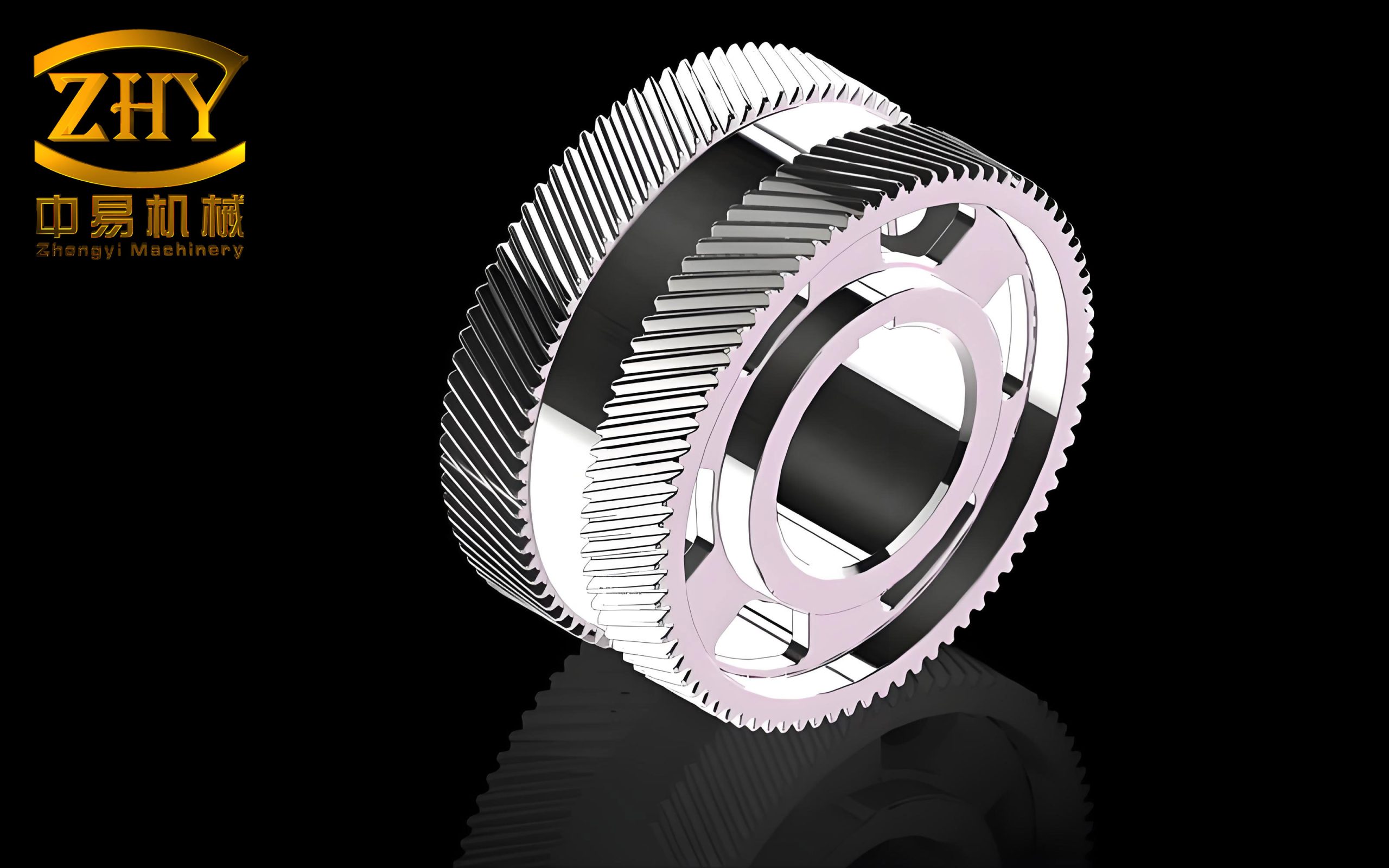
Modern mechanical equipment is rapidly advancing toward heavy-duty, high-precision, and high-speed operation, imposing ever-increasing performance requirements on mechanical transmission systems. Among various transmission forms, gear transmission remains the most widely used due to its reliability, compactness, and high efficiency. Within this domain, the herringbone gear, also known as a double-helical gear, combines the advantages of both spur and helical gear transmissions. It provides stable and reliable power transfer, reduced impact and noise, and critically eliminates the axial thrust forces that plague conventional helical gears under heavy loads. These characteristics make herringbone gears particularly suitable for demanding applications in marine propulsion, aerospace power transmission, heavy machinery, and other critical industrial sectors where both high load capacity and transmission accuracy are paramount.
However, during the manufacturing process of herringbone gears, various errors inevitably arise. Unlike standard helical gears, the herringbone gear comprises two oppositely handed helical tooth flanks joined at a central plane. This unique double-helix configuration introduces additional complexity, including a critical alignment error at the center plane. Furthermore, both the left-hand and right-hand tooth flank errors must be independently considered. These errors, including tooth profile deviations, helix deviations, pitch deviations, and the characteristic herringbone alignment error, all contribute to transmission error (TE) in the gear system, directly degrading the stability and positional accuracy of the entire drivetrain. Understanding and quantifying how these manufacturing errors affect transmission accuracy is essential for improving gear quality and overall system performance.
Therefore, the primary objective of this research is to establish a comprehensive mathematical model capable of predicting the transmission accuracy of herringbone gear systems while explicitly accounting for measured manufacturing errors. To address the complexity of the three-dimensional double-helix geometry, I employ a slice method that discretizes the gear into a series of thin slices along the face width. Based on this discretization, I establish deformation compatibility conditions and formulate the equations of motion to solve for the resulting transmission error. Additionally, I integrate equivalent error gaps derived from actual gear measurements into the model to analyze the influence of each manufacturing error category. The model’s validity is confirmed through dedicated experiments on a pair of manufactured five-grade precision herringbone gears. Finally, I extend this slice-based methodology to herringbone planetary gear systems, providing a comprehensive framework for evaluating transmission accuracy across different gear architectures.
2. Characterization and Equivalence of Manufacturing Errors for Herringbone Gears
2.1 Definition and Classification of Key Error Components
To effectively model the influence of manufacturing errors, I first delineate the specific error components identified in gear metrology standards, adapted for the herringbone gear geometry.
(1) Tooth Profile Deviation
Tooth profile deviation represents the amount by which the actual tooth profile deviates from the ideal involute profile within the evaluation range. It encompasses:
- Total profile deviation (Fα): The distance between two design profile lines that enclose the actual profile within the profile evaluation range.
- Profile form deviation (ffα): The distance between two curves of identical shape to the mean profile enclosing the actual profile.
- Profile slope deviation (fHα): The distance between two design profile lines intersecting the endpoints of the mean profile.
(2) Helix (Tooth Trace) Deviation
This family of errors describes deviations along the tooth width direction and is critical for load distribution uniformity. It includes:
- Total helix deviation (Fβ): The distance between two design helix lines enclosing the actual helix line within the evaluation range.
- Helix form deviation (ffβ): Distance between two curves identical in shape to the mean helix enclosing the actual helix.
- Helix slope deviation (fHβ): Distance between two design helix lines intersecting the mean helix endpoints.
(3) Pitch Deviation
Pitch deviations primarily affect the accuracy of motion transfer and smoothness of operation.
- Single pitch deviation (fpt): The algebraic difference between the actual pitch and the theoretical pitch measured on a circle near mid-tooth height.
- Cumulative pitch deviation (Fpk): The algebraic difference between the actual arc length and theoretical arc length over any k pitches.
- Total cumulative pitch deviation (Fp): The total amplitude of the cumulative pitch deviation curve over the entire gear circumference.
(4) Alignment Error
This error is unique to herringbone gears due to their construction from two oppositely handed helical halves. The alignment error quantifies the deviation of the intersection point of the left-hand and right-hand tooth flanks from the ideal central plane. It is defined by the axial deviation ΔTh, circumferential deviation ΔTs, and normal deviation ΔTn. These are interrelated through the helix angle β:
$$ f = \frac{2 \cdot \Delta T_s}{\tan \beta} = 2 \cdot \Delta T_h \tag{2.1} $$
$$ \Delta T_s = \frac{2 \cdot \Delta T_n}{\sin 2\beta} \tag{2.2} $$
2.2 Fitting of Measured Error Surfaces and Curves
To accurately reflect the true manufacturing state of the herringbone gear, I utilize measurement data obtained from a Klingelnberg P100 gear measuring machine. The discrete measurement points for tooth profile and helix deviations are fitted using a bi-cubic B-spline interpolation algorithm to reconstruct the actual error surface for each flank.
The surface fitting process involves constructing a control points grid from the measured data, with points arranged in (n+1) rows and (m+1) columns across the profile and face width directions, respectively. A cubic B-spline curve is first fitted along one direction, followed by another fitting pass along the orthogonal direction, resulting in a smooth, interpolated error surface. This captured surface represents the combined effect of both profile and helix errors at every point on the tooth flank, providing a detailed and realistic input for subsequent transmission error analysis.
Following the surface reconstruction, the measured cumulative pitch error data are processed to create a piecewise function representing the error for each individual tooth. Similarly, the alignment error values measured at each tooth position are fitted to form a continuous error curve. These fitted datasets provide the foundation for equivalent error gap calculation.
Table 2.1: Measured herringbone gear error data categories
| Error Category | Measurement Instrument | Data Form | Application in Model |
|---|---|---|---|
| Tooth profile & helix error | Klingelnberg P100 | 3D surface (via B-spline fitting) | Position-dependent error gaps |
| Pitch error | Klingelnberg P100 | Piecewise function over tooth number | Tooth-index-dependent error per contact |
| Alignment error | Coordinate Measuring Machine | Fitted curve per tooth | Initial backlash and relative flank shift |
2.3 Equivalence of Manufacturing Errors to Contact Spring Gaps
To embed the measured errors into the transmission accuracy model, I transform them into equivalent gaps along the common normal direction of the contacting tooth flanks. This transformation allows the errors to be treated as initial separations in the contact spring system.
(1) Tooth Profile and Helix Errors
Using the fitted error surface, defined as a function z = G(p, q) where p represents the face width coordinate and q represents the profile radius coordinate, the error gap ej at any meshing point can be determined. The meshing point radius r(Pi) is first calculated from the gear geometry. Then, the corresponding error value is extracted from the surface and projected onto the normal direction:
$$ e_{j}^{b} = G\left(l(j), r(P_i)\right) \cdot \cos \beta_b \tag{2.8} $$
where l(j) is the axial coordinate of the j-th slice, and βb is the base helix angle.
(2) Pitch Errors
For a set of simultaneously meshing tooth pairs, the pitch error is indexed by the specific tooth number. The equivalent gap on the meshing line is:
$$ e_{p}^{t} = F[s(w)] \cdot \cos \beta_b \cdot \cos \alpha_t \tag{2.10} $$
where F[s(w)] is the cumulative pitch error for tooth number s, αt is the transverse pressure angle.
(3) Alignment error
The presence of alignment error causes an axial floatation and a slight rotation of one gear relative to the other as the gears seek a stable equilibrium contact position. This movement results in an additional gap on one helix side while the other side achieves contact. The equivalent additional gap due to alignment error is determined by analyzing the contact line positions on the meshing plane after the float has occurred. The resulting gap can be expressed as:
$$ e_{m}^{b} = (\lambda_m \cdot \tan \beta_b – \lambda_m’) \cos \beta_b \tag{2.11} $$
where λm represents the alignment error value for the m-th gear, λ̄’m is the minimum error among the simultaneously meshing teeth of both flanks, and the terms account for the axial and circumferential components of the error.
3. Transmission Accuracy Model for a Pair of Herringbone Gears
3.1 Slice Discretization Method
The herringbone gear, characterized by its double-helix structure, presents a complex three-dimensional meshing scenario. To manage this complexity, I adopt a slice discretization approach. The gear pair is virtually divided into a series of thin, independent slices along the face width direction. Each slice, due to its infinitesimal thickness, can be effectively modeled as a spur gear. This simplifies the three-dimensional contact problem into a set of manageable two-dimensional planar contact problems, as illustrated in the conceptual model.
For the j-th slice, the relative angular displacement between the local slice coordinate system and the base coordinate system is:
$$ \Delta \beta_{Jj} = \Delta l \cdot \left( \frac{l}{r_J \cdot n} \right) \cdot \tan \beta, \quad J \in \{p, g\} \tag{3.1} $$
where l is the total face width, n is the number of slices, and rJ are the pitch radii. At any given meshing instant, only a subset of these slices are in active contact, determined by the position of the instantaneous contact lines on the meshing plane.
3.2 Calculation of Meshing Stiffness
The single-tooth mesh stiffness for each slice is calculated using the potential energy method, which decomposes the total strain energy into components from Hertzian contact, bending, shear, axial compression, and gear body flexibility.
For a spur gear slice, the bending stiffness kb, shear stiffness ks, and axial compressive stiffness ka are derived by modeling the tooth as a variable cross-section cantilever beam:
$$ \frac{1}{k_b} = \int_{-\alpha_1}^{\alpha_2} \frac{3(1 + \cos \alpha_1 (\alpha_2 – \alpha) \cos \alpha)^2(\alpha_2 – \alpha) \cos \alpha}{2 E l \left[ \sin \alpha + (\alpha_2 – \alpha) \cos \alpha \right]^3} \, d\alpha \tag{3.9} $$
$$ \frac{1}{k_s} = \int_{-\alpha_1}^{\alpha_2} \frac{1.2(1 + u)(\alpha_2 – \alpha) \cos \alpha \cos^2 \alpha_1}{E l \left[ \sin \alpha + (\alpha_2 – \alpha) \cos \alpha \right]} \, d\alpha \tag{3.10} $$
$$ \frac{1}{k_a} = \int_{-\alpha_1}^{\alpha_2} \frac{(\alpha_2 – \alpha) \cos \alpha \sin^2 \alpha_1}{2 E l \left[ \sin \alpha + (\alpha_2 – \alpha) \cos \alpha \right]} \, d\alpha \tag{3.11} $$
The gear body flexibility stiffness kf is calculated using the theory developed by Sainsot et al., which accounts for the elastic deformation of the gear rim structure. Finally, the Hertzian contact stiffness kh is treated as a constant for a given gear width and material, based on the well-known Hertzian contact theory.
The total mesh stiffness for the j-th slice of a gear pair is obtained by combining the individual stiffness components for both the driving (p) and driven (g) gears in series:
$$ \frac{1}{k_{pg,j}^{L/R}} = \frac{1}{k_{b,p}} + \frac{1}{k_{s,p}} + \frac{1}{k_{a,p}} + \frac{1}{k_{f,p}} + \frac{1}{k_{b,g}} + \frac{1}{k_{s,g}} + \frac{1}{k_{a,g}} + \frac{1}{k_{f,g}} + \frac{1}{k_{h}} \tag{3.17} $$
3.3 Establishment of the Transmission Accuracy Model
(1) Coordinate System Definition
I establish a global coordinate frame (OXYZ) at the center of the driving gear and a secondary frame at the driven gear center (OgXgYgZg). Each gear is considered as a rigid body with six degrees of freedom: three translational displacements (x, y, z) and three rotational displacements around these axes. The generalized displacement vector X for the entire gear pair system is defined as:
$$ X = (x_p, y_p, z_p, u_{px}, u_{py}, u_{pz}, x_g, y_g, z_g, u_{gx}, u_{gy}, u_{gz})^T \tag{3.18} $$
(2) Deformation Compatibility Conditions
The elastic deformation δL/Rpg,j for each slice is the relative displacement of the gear centers projected onto the contact normal direction minus the error gap. The mesh deformation for the left (L) and right (R) helix flanks is mathematically expressed as:
$$ \delta_{pg,j}^{L/R} = n^{L/R} \cdot X – e_{pg,j}^{L/R} \tag{3.19a} $$
where nL/R is the projection vector of the 12-degree-of-freedom motion along the contact normal, and eL/Rpg,j is the total equivalent error gap for that slice. The mesh is active only when the deformation is positive. The associated mesh stiffness is then:
$$ k_{pg,j}^{L/R} = \begin{cases} k_{pg,j}^{L/R}, & \delta_{pg,j}^{L/R} > 0 \\ 0, & \delta_{pg,j}^{L/R} \le 0 \end{cases} \tag{3.19b} $$
The projection vector is a function of the base helix angle βb, the transverse pressure angle αt, the base radii of the gears (rb1, rb2), and the position on the meshing line. The projection vector nL/R for the external gear pair is given in Eq. (3.20). This vector decomposes the relative translation and rotation of each gear into the component that influences the meshing along the line of action.
(3) Equations of Motion and Solution
The equations of motion for the gear pair system, in matrix form, are given by:
$$ (K_m + K_h) X = F + T \tag{3.26} $$
where:
- Km is the global meshing stiffness matrix, assembled from the individual slice stiffnesses and projection vectors: Km = KmL + KmR.
- Kh is the support stiffness matrix, representing the bearing and foundation stiffness in all six directions at each gear center.
- F is the vector of equivalent excitation forces due to the manufacturing errors.
- T is the vector of external applied torques.
By solving the linear algebraic system, the generalized displacement vector X is obtained. The transmission error, a key metric of gear accuracy, is defined as the difference between the actual output angular position and the theoretical output position. Since the input rotary inertia is fixed, the transmission error (unit: arc-seconds) is directly derived from the driven gear’s rotational displacement along the z-axis:
$$ TE = \frac{180 \cdot 3600}{\pi} \cdot u_{gz} \tag{3.27} $$
(4) Error Inclusion
The total error gap eL/Rpg,j for each slice integrates the equivalent gaps from tooth profile (eα), tooth pitch (ep), and alignment errors. The individual error components are modeled as described in detail in Section 2.3.
3.4 Analysis of Single Error Effects
Utilizing the parameterized model, I investigate the influence of individual manufacturing errors on the transmission accuracy of the herringbone gear pair. The basic parameters for the analysis are presented in Table 3.1.
Table 3.1: Basic parameters of the gear pair for simulation
| Parameter | Driving Gear | Driven Gear |
|---|---|---|
| Number of teeth | 25 | 50 |
| Normal module (mm) | 4 | 4 |
| Normal pressure angle (°) | 20 | 20 |
| Helix angle (°) | 20 | 20 |
| Face width (mm) | 52 | 48 |
(1) Influence of Tooth Profile Error
Tooth profile error is simulated as a harmonic function varying at the gear mesh frequency, and its effect on transmission error is depicted in Figure 3.1. In this figure, the transmission error is plotted against the rotation angle of the driven gear for different gear accuracy grades. The analysis reveals several key insights:
- Increasing the magnitude of the profile error from grade 4 to grade 6 leads to an increase in the amplitude of the transmission error.
- Examination of an individual curve shows a high-frequency oscillation superimposed on the transmission error curve. This oscillation is a direct consequence of the profile error varying along the involute profile, which affects the instantaneous contact point and thus the effective kinematic relationship. This results in periodic fluctuations that directly impact the gear’s rotational accuracy.
(2) Influence of Pitch Error
Pitch error, being an accumulated error, is modeled as a sinusoidal function over one full rotation of the gear. The influence of pitch error on the transmission error is shown in Figure 3.2. The analysis demonstrates:
- Pitch error contributes a substantial, low-frequency, sinusoidal variation to the transmission error over one full revolution of the gear.
- Additionally, a distinct step-like change in the transmission error is observed at the moment a new tooth pair enters or exits the meshing zone. This is because the pitch error alters the rotational phase between successive tooth engagements, causing discontinuities in the output angle.
- Similar to before, the magnitude of these error characteristics is directly proportional to the total cumulative pitch error as defined by the gear precision grade.
3.5 Monte Carlo Analysis of Manufacturing Tolerances
To predict the statistical distribution of transmission error, I employ the Monte Carlo simulation method. This technique treats manufacturing errors as random variables with specific probability distributions. According to theory and empirical evidence:
- Tooth profile error (Fα) and total cumulative pitch error (Fp) are primarily generated by geometric and kinematic eccentricities in the manufacturing process and are assumed to follow a Rayleigh distribution.
- Helix error (Fβ), being a measure of form and position error along the tooth trace, typically follows a Normal distribution.
The parameters for these distributions are derived from the corresponding tolerance values for each precision grade (Table 3.2). By statistically sampling these error distributions and running the transmission accuracy model multiple times, I obtain a distribution of possible transmission error values, which is then analyzed statistically.
Table 3.2: Tolerance values used in Monte Carlo analysis (mm)
| Precision Grade | F_α (Pinion) | F_α (Gear) | F_p (Pinion) | F_p (Gear) | F_β (Pinion) | F_β (Gear) |
|---|---|---|---|---|---|---|
| 4 | 0.0065 | 0.0075 | 0.014 | 0.018 | 0.006 | 0.0065 |
| 5 | 0.0095 | 0.011 | 0.019 | 0.025 | 0.0085 | 0.009 |
| 6 | 0.013 | 0.015 | 0.028 | 0.036 | 0.012 | 0.013 |
The statistical parameters of the maximum transmission error for each precision grade are summarized below. This provides a clear and quantitative prediction of the achievable transmission accuracy for a given manufacturing tolerance.
Table 3.3: Statistical results of transmission error from Monte Carlo simulation
| Precision Grade | Mean TE (“) | Standard Deviation σ(“) | 99.7% Confidence Interval (“) |
|---|---|---|---|
| 4 | 14.06 | 10.64 | [6.54, 25.18] |
| 5 | 19.25 | 19.80 | [8.95, 33.57] |
| 6 | 26.94 | 41.37 | [12.30, 48.91] |
The results show a clear trend: as the precision grade worsens, the mean transmission error, its standard deviation, and the confidence interval width all increase. This indicates not only a loss in accuracy but also a reduction in consistency and predictability of the gear pair’s performance.
4. Experimental Verification of the Herringbone Gear Transmission Accuracy Model
4.1 Gear Design and Manufacturing Error Detection
To validate the theoretical model, I designed and manufactured a pair of 5-grade precision herringbone gears. The specifications of these gears are presented in Table 4.1. The manufacturing errors were subsequently measured using a Klingelnberg P100 gear measuring machine and a precision coordinate measuring machine.
Table 4.1: Parameters of the experimental herringbone gear pair
| Specification | Pinion | Gear |
|---|---|---|
| Number of teeth | 25 | 50 |
| Normal module (mm) | 4 | 4 |
| Helix angle (°) | 19.37 | 19.37 |
| Normal pressure angle (°) | 20 | 20 |
| Face width (mm) | 52 | 48 |
| Tooth thickness (mm) | 6.283-0.11-0.151 | 6.283-0.11-0.159 |
| Material | 12Cr2Ni4, carburized & quenched | |
The measured errors were then used as inputs to the transmission accuracy model. The model’s predictions for both the combined effects of all errors and the isolated effect of the tooth surface error (profile + helix) were computed.
4.2 Test Setup and Methodology
The experimental validation was conducted on a dedicated gear transmission test rig. The test bench comprises a servo motor, a reducer, a pair of test herringbone gears, high-precision angle encoders on both input and output shafts, a torque sensor, and a magnetic powder brake for loading. The gears were mounted in a cantilever arrangement on the shafts. The measured torque and speed conditions for the experiments are summarized in Table 4.2.
Table 4.2: Test conditions
| Condition | Input Torque (N·m) | Input Speed (rpm) |
|---|---|---|
| 1 | 0 | 2 |
| 2 | 50 | 2 |
| 3 | 100 | 2 |
The transmission error was calculated by comparing the actual measured output angle, as recorded by the output encoder, with the theoretical output angle derived from the input encoder reading and the gear ratio:
$$ TE = \theta_{out} – \frac{\theta_{in}}{i} \tag{4.3} $$
Table 4.3: Simulation vs. experimental TE amplitude comparison
| Input Torque (N·m) | Simulated TE (“) | Experimental TE (“) | Relative Error (%) |
|---|---|---|---|
| 0 | 62.6 | 67.8 | -7.7 |
| 50 | 57.98 | 65.38 | -11.3 |
| 100 | 54.8 | 64.57 | -15.2 |
The comparison between the simulated and experimental transmission error curves shows good agreement. The overall waveform shape, including the low-frequency sinusoidal variation and the high-frequency ripples, matches well. As detailed in Table 4.3, the differences in TE amplitudes between simulation and experiment are within 16% for all torque conditions. Several factors contribute to the observed discrepancies. These include possible measurement errors in the angle encoders, manual errors in assessing the installation alignment of the test rig, surface roughness effects not accounted for in the model, and other random deviations in the manufacturing process. These results demonstrate the accuracy and practical applicability of the developed model.
5. Extension to Herringbone Planetary Gear Transmission
5.1 System Model and Deformation Compatibility
Building upon the validated model for a single gear pair, I extend the slice method to a more complex herringbone planetary gear system. This system, as modeled, consists of a central sun gear (s), a carrier (c) that provides the output, and three planetary gears (pi) that mesh with both the sun gear and a fixed internal ring gear (r). The displacement vector and the equations of motion are formulated on the same basis as the simple gear pair, but the matrices are expanded to account for the interaction between the sun gear and each planet, and between each planet and the ring gear.
Each gear in the system is again modeled as a rigid body with 6 degrees of freedom, giving the entire system a total of (3+N)×6 degrees of freedom, where N is the number of planets.
The mesh deformations for the sun-planet (spi) and planet-ring (rpi) contacts are calculated based on the relative displacements of the gear centers projected on the respective lines of action. The projection vectors for these internal and external meshes account for the geometry and orientation of each gear, similar to the approach used for the simple gear pair. The deformation coordinates for the left flank of the external mesh (sun-planet) are given by:
$$ \delta_{sp_i,j}^{L} = n_{Ei}^{L} \cdot [x_s, y_s, z_s, u_{sx}, u_{sy}, u_{sz}, x_{p_i}, y_{p_i}, z_{p_i}, u_{p_ix}, u_{p_iy}, u_{p_iz}]^T – e_{sp_i,j}^{L} \tag{5.3} $$
Similarly, for the internal mesh (planet-ring):
$$ \delta_{rp_i,j}^{L} = n_{Ii}^{L} \cdot [x_r, y_r, z_r, u_{rx}, u_{ry}, u_{rz}, x_{p_i}, y_{p_i}, z_{p_i}, u_{p_ix}, u_{p_iy}, u_{p_iz}]^T – e_{rp_i,j}^{L} \tag{5.6} $$
The system’s equations of motion are written as:
$$ (K_m + K_h) X = F + T \tag{5.9} $$
where Kh is the support stiffness matrix, Km is the combined mesh stiffness matrix, F is the internal excitation vector from errors, and T is the external torque vector. The structure of the stiffness matrix Km is elaborated, showing the coupling between the sun gear, ring gear, carrier, and planets.
Table 5.1: Parameters for the herringbone planetary gear system simulation
| Component | Number of Teeth | Module (mm) | Pressure Angle (°) | Helix Angle (°) | Face Width (mm) |
|---|---|---|---|---|---|
| Sun Gear | 22 | 16 | 20 | 25 | 100 |
| Planet Gear | 41 | 16 | 20 | 25 | 100 |
| Ring Gear | 104 | 16 | 20 | 25 | 100 |
5.2 Influence of Manufacturing Errors on Planetary System Accuracy
Using the established planetary gear model, I analyzed the influence of tooth profile errors and pitch errors on the overall system transmission error.
(1) Impact of Tooth Profile Error
When the profile error is introduced to only one gear component at a time, the planetary gear (planet) has the most significant effect on the system’s transmission error amplitude. This is followed by the ring gear and then the sun gear. The reason is that the planet gear participates in two meshing actions (one with the sun and one with the ring) during a single carrier rotation, thus transmitting errors from both meshes directly to the output. The sun gear only contributes via the external mesh, while the ring gear only influences the internal mesh. When all gears have profile errors simultaneously, the overall system transmission error amplitude further increases, as shown in Figure 5.4 (b), highlighting the compound effect of errors from multiple sources.
(2) Impact of Pitch Error
Similarly, when pitch errors are introduced, the same hierarchy is observed: the planet gear has the greatest individual impact, followed by the ring gear and then the sun gear. This confirms that the gear which participates in multiple meshing paths is the most critical for precision in a planetary system. Simultaneously introducing pitch errors to all gears results in the largest overall transmission error, as the errors from sun-planet and planet-ring meshes are superimposed.
5.3 Monte Carlo Simulation for Planetary Gear System
I further conducted a Monte Carlo simulation for the planetary gear system to assess the statistical distribution of its transmission error under different manufacturing precision grades. The tolerance values for the sun, planet, and ring gears at grades 4, 5, and 6 are presented in Table 5.2.
Table 5.2: Error tolerance values for planetary system components (mm)
| Error | Component | Grade 4 | Grade 5 | Grade 6 |
|---|---|---|---|---|
| F_α | Sun | 0.012 | 0.016 | 0.023 |
| Planet | 0.013 | 0.018 | 0.026 | |
| Ring | 0.014 | 0.020 | 0.031 | |
| F_p | Sun | 0.025 | 0.036 | 0.050 |
| Planet | 0.032 | 0.045 | 0.064 | |
| Ring | 0.047 | 0.067 | 0.094 | |
| F_β | Sun | 0.009 | 0.013 | 0.018 |
| Planet | 0.0095 | 0.014 | 0.019 | |
| Ring | 0.011 | 0.015 | 0.022 |
Simulations were run 6000 times for each precision grade. The resulting maximum transmission error distributions were statistically analyzed, and the findings are summarized in Table 5.3.
Table 5.3: Statistical results of planetary system transmission error
| Precision Grade | Mean TE (“) | Standard Deviation σ(“) | 99.7% Confidence Interval (“) |
|---|---|---|---|
| 4 | 57.54 | 236.82 | [22.09, 113.42] |
| 5 | 81.22 | 471.06 | [81.22, 155.90] |
| 6 | 115.06 | 931.40 | [43.94, 223.57] |
The simulation results reveal a significant increase in transmission error for the planetary system compared to a simple gear pair operating under the same precision grade. This is expected because the planetary system has multiple meshing paths, and errors from each gear (sun, ring, and planet) contribute to the final output. The standard deviation increases substantially with a lower precision grade, indicating that the error accumulation effect is more pronounced and less predictable in complex multi-stage transmission systems.
Conclusions
This thesis presents a comprehensive investigation into the modeling and analysis of herringbone gear transmission accuracy, explicitly accounting for the effects of manufacturing errors. The key contributions and findings are as follows:
(1) Comprehensive Error Characterization and Equivalence: I successfully characterized key manufacturing errors, including tooth profile, helix, pitch, and the unique herringbone alignment error. A method was developed to fit actual measured 3D error surfaces using bi-cubic B-splines and to equivalently transform all these errors into effective contact spring gaps along the tooth normal direction, enabling their integration into a mechanical model.
(2) Development of a Slice-Based Transmission Accuracy Model: A novel transmission accuracy model for a pair of herringbone gears was established using the slice discretization method. This model effectively balances accuracy and computational efficiency by simplifying the 3D contact problem into a series of 2D problems. The model successfully simulates the influence of manufacturing errors and forms the basis for a more complex system model.
(3) Analysis of Error Impacts and Statistical Prediction: The model was used to analyze the distinct signatures of each error type. Tooth profile errors cause high-frequency ripples; pitch errors lead to large-scale sinusoidal patterns and step changes; and alignment errors produce step-like variations in transmission error. A Monte Carlo simulation method was employed to statistically predict the transmission error ranges for different manufacturing precision grades, offering a powerful tool for design and quality assurance.
(4) Experimental Validation: The accuracy and feasibility of the slice-based model were confirmed through a dedicated transmission error experiment on a pair of 5-grade precision herringbone gears. The comparison between simulation and experimental results showed good agreement, with the transmission error amplitude differences being within 16% across various torque conditions. The experimental waveform confirmed the mathematical model’s ability to capture both the macro-periodic and micro-oscillatory characteristics of gear transmission error.
(5) Extension to Planetary Gear Systems: The general methodology was successfully extended to model the transmission accuracy of a herringbone planetary gear system. The model identified the planet gear as the most critical component influencing system accuracy, as it participates in multiple meshing paths. Statistical analysis using the Monte Carlo method clarified how manufacturing error tolerances of all components affect the overall planetary system’s precision, providing a basis for error allocation and quality control in complex gear systems.
The models and analytical methods developed in this research provide a robust framework for predicting, evaluating, and controlling the transmission accuracy of herringbone gears and their planetary systems under the influence of manufacturing errors. This contributes significantly to the production of high-performance and high-precision herringbone gear drivetrains. The current work opens avenues for future research, including the integration of tooth profile and helix modifications into the model to study their potential in mitigating the adverse effects of manufacturing errors.