
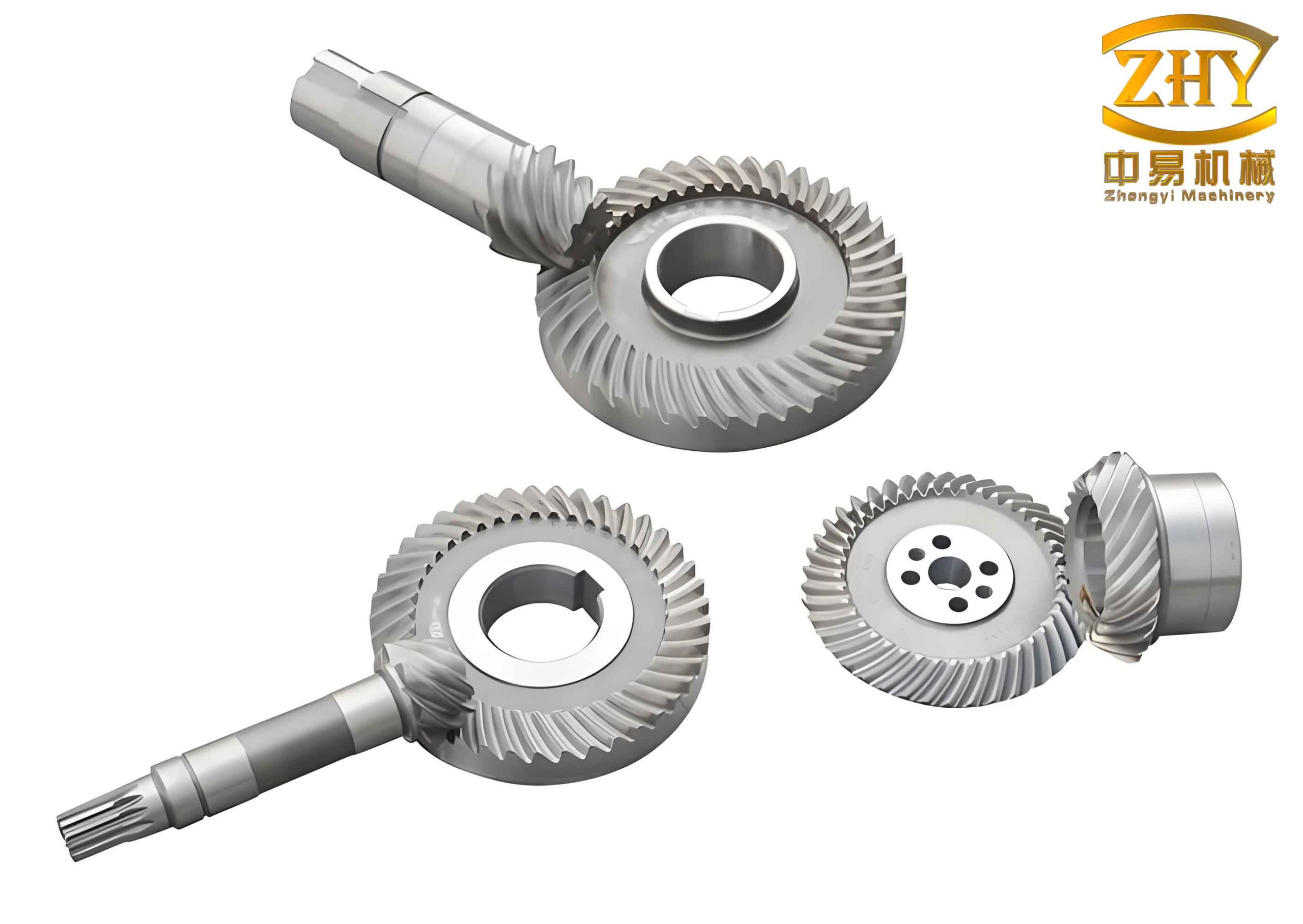
In modern power transmission systems, particularly within automotive drivetrains, robotics, and aerospace applications, hyperboloid gears are prized for their unique capabilities. Their defining feature, the offset between the axes of the driving and driven gears, allows for more compact and flexible design configurations. Furthermore, they offer high contact ratios, smooth torque transfer, and inherent tolerance to certain dynamic loads. However, the very geometry that grants these advantages also makes their meshing performance—specifically the contact pattern and transmission error—exceptionally sensitive to small deviations from their ideal assembled position. These deviations, known as assembly misalignments or installation errors, are unavoidable in real-world manufacturing and assembly processes. They can lead to edge loading, increased vibration and noise, accelerated wear, and reduced gear life. Therefore, developing hyperboloid gears with inherently low sensitivity to such misalignments is a critical engineering challenge. This article presents a comprehensive methodology for the optimal design of hyperboloid gears to achieve robust meshing performance in the presence of assembly errors.
The core of the problem lies in controlling the tooth contact characteristics. Traditional design methods often result in a contact pattern and transmission error function that are optimal only under perfect alignment. When misalignments occur, the contact ellipse can shift dramatically towards the tooth edges, and the amplitude of transmission error can increase, becoming a primary source of gear whine. While previous research has extensively analyzed the impact of misalignments and optimized parameters like machine-tool settings, there remains a need for a holistic optimization framework. This framework should directly link pre-designed contact parameters, through an efficient contact analysis model, to a quantitative measure of sensitivity against the full spectrum of assembly errors, and then minimize this sensitivity.
The proposed methodology is built upon several interconnected pillars: a quantitative model for evaluating contact characteristics under misalignment, an efficient numerical model for Tooth Contact Analysis (TCA) using Non-Uniform Rational B-Spline (NURBS) surface representation, a sensitivity analysis model, and finally, a multi-objective optimization routine. The goal is to systematically alter the fundamental geometry of the hyperboloid gears to make their performance more forgiving to assembly variations.
1. Quantitative Evaluation of Contact Characteristics Under Misalignment
To assess and ultimately optimize performance, one must first define quantifiable metrics that describe the gear meshing quality. For hyperboloid gears, three key characteristics are paramount: the location and size of the contact pattern, and the shape of the transmission error curve. Under the influence of assembly misalignments, these characteristics deviate from their designed state. We define four specific assembly error components according to standard practice:
$$ \Delta Z_p : \text{Pinion axial error.} $$
$$ \Delta X_g : \text{Gear axial error.} $$
$$ \Delta E : \text{Offset error.} $$
$$ \Delta \Sigma : \text{Shaft angle error.} $$
The change in contact properties due to these errors is evaluated using the following models.
1.1 Variation of Contact Area ($\Delta S_{cp}$)
The contact area $S_{cp}$ is a critical indicator of load distribution and contact stress. A large, centrally located area is desirable. Under misalignment, this area can shrink or distort. We calculate the contact area by discretizing the contact pattern boundary formed by the endpoints of the instantaneous contact ellipses along the path of contact. The area of the polygon formed by these discrete points $(x_i, y_i)$ is computed using the shoelace formula. The change in contact area is:
$$ \Delta S_{cp} = S_{cp}^{(e)} – S_{cp}^{(0)} = f_S(\Delta Z_p, \Delta X_g, \Delta E, \Delta \Sigma) $$
where $S_{cp}^{(0)}$ is the area under perfect alignment and $S_{cp}^{(e)}$ is the area under misalignment.
1.2 Shift of Contact Path Center ($\Delta x_{cp}, \Delta y_{cp}$)
The center of the contact path indicates where the load is primarily carried on the tooth flank. A significant shift can lead to edge contact. The coordinates of the center point $(x_{cp}, y_{cp})$ are calculated as the area-weighted centroid of the contact pattern polygon:
$$ x_{cp} = \frac{1}{S_{cp}} \sum_{i=1}^{n-1} \left( \frac{x_{a_i} + x_{a_{i+1}} + x_{b_i} + x_{b_{i+1}}}{4} \right) S_i $$
$$ y_{cp} = \frac{1}{S_{cp}} \sum_{i=1}^{n-1} \left( \frac{y_{a_i} + y_{a_{i+1}} + y_{b_i} + y_{b_{i+1}}}{4} \right) S_i $$
The shift due to misalignment is:
$$ \Delta x_{cp} = x_{cp}^{(e)} – x_{cp}^{(0)} = f_x(\Delta Z_p, \Delta X_g, \Delta E, \Delta \Sigma) $$
$$ \Delta y_{cp} = y_{cp}^{(e)} – y_{cp}^{(0)} = f_y(\Delta Z_p, \Delta X_g, \Delta E, \Delta \Sigma) $$
1.3 Change in Transmission Error Fluctuation Amplitude ($\Delta TE$)
Transmission error (TE) is the primary excitation source for gear noise. A parabolic function with minimal amplitude is often targeted for low noise. The amplitude, typically measured at the “knee” or transition point of the TE curve over one mesh cycle, is denoted as $TE$. Misalignments can drastically increase this amplitude. The change is defined as:
$$ \Delta TE = TE^{(e)} – TE^{(0)} = f_{TE}(\Delta Z_p, \Delta X_g, \Delta E, \Delta \Sigma) $$
Minimizing $\Delta TE$ is crucial for maintaining acoustic performance under real assembly conditions.
2. Efficient TCA Model Using NURBS Surface Fitting
To analyze the relationship between gear geometry, misalignment, and the contact metrics defined above, an efficient Tooth Contact Analysis (TCA) model is essential. Traditional TCA involves solving complex nonlinear equations derived from the gear tooth surfaces, which can be computationally intensive and sensitive to initial guesses. We employ a method that uses NURBS surfaces to accurately represent the pinion tooth flank, significantly simplifying the contact simulation.
2.1 Gear Geometry Definition via Local Synthesis
The starting point is the definition of the gear pair geometry using the local synthesis method. This method allows for direct pre-specification of the contact conditions at a designated reference point on the tooth flank. The key pre-set parameters are:
$$ m_{21}’ : \text{First derivative of transmission ratio (slope of transmission error).} $$
$$ a : \text{Semi-major axis length of the contact ellipse at the reference point.} $$
$$ \eta_2 : \text{Angle between the contact path and the root line on the gear tooth.} $$
These parameters $m_{21}’$, $a$, and $\eta_2$ fundamentally control the local curvature and orientation of the pinion tooth surface relative to the gear. Through the principles of differential geometry and gear meshing, a set of equations (the basic equations of local synthesis) are solved to determine the principal curvatures and directions at the reference point. Subsequently, these geometric parameters are used to calculate the actual machine-tool settings (e.g., cutter tilt, swivel angle, radial distance) required to generate the pinion tooth surface via a face-hobbing or face-milling process. The mathematical relationship can be summarized as:
$$ \mathbf{F}(m_{21}’, a, \eta_2, \,\, X_{g1}, X_{b1}, S_{r1}, E_1, q, \alpha_t, \alpha_r, \gamma_1) = 0 $$
where the latter terms are the specific machine setting parameters.
2.2 NURBS Surface Fitting of the Pinion Flank
The theoretical pinion surface, generated by the machine tool equations, is typically defined by three parameters: a cutter surface parameter, a rotation angle parameter, and the work gear rotation angle. Direct TCA using this parameterization is inefficient. We approximate this surface with a NURBS patch, which is defined by only two parameters ($u$, $v$) corresponding to the profile and lengthwise directions. A NURBS surface of degree 3 is given by:
$$ \mathbf{P}(u,v) = \frac{\sum_{i=0}^{m} \sum_{j=0}^{n} w_{i,j} \mathbf{d}_{i,j} N_{i,3}(u) N_{j,3}(v)}{\sum_{i=0}^{m} \sum_{j=0}^{n} w_{i,j} N_{i,3}(u) N_{j,3}(v)} $$
where $\mathbf{d}_{i,j}$ are control points, $w_{i,j}$ are weights, and $N_{i,3}(u)$ are the B-spline basis functions. The fitting process involves sampling points from the theoretical surface, constructing knot vectors using chord-length parameterization, and solving for the control points and weights. This results in a highly accurate mathematical model of the pinion tooth flank with greatly reduced parametric complexity. The accuracy is validated by ensuring the fitting error is within an acceptable limit (e.g., on the order of $10^{-3}$ mm).
2.3 Contact Analysis with Misalignment
With the gear tooth surface represented in closed form and the pinion surface represented as a NURBS patch, the TCA conditions are enforced. The fundamental requirement for contact is that the position vectors and surface normals of both gears coincide at the contact point in a common coordinate system, considering the relative position imposed by the assembly errors. The condition for continuous tangency during rotation adds the requirement that the relative velocity lies in the common tangent plane. These conditions yield a system of five nonlinear equations:
$$ \mathbf{r}_1^{(n)}(u, v, \phi_1, \Delta) = \mathbf{r}_2^{(n)}(s, \theta, \phi_2, \Delta) $$
$$ \mathbf{n}_1^{(n)}(u, v, \phi_1) = \mathbf{n}_2^{(n)}(s, \theta, \phi_2) $$
$$ \mathbf{n}_1^{(n)} \cdot \mathbf{v}_{12}^{(n)} = 0 $$
Here, $\mathbf{r}$ and $\mathbf{n}$ denote position and unit normal vectors, subscripts 1 and 2 refer to pinion and gear, $(u,v)$ and $(s,\theta)$ are respective surface parameters, $(\phi_1, \phi_2)$ are rotation angles, and $\Delta$ represents the set of assembly errors $(\Delta Z_p, \Delta X_g, \Delta E, \Delta \Sigma)$. Solving this system for a sequence of pinion rotation angles $\phi_1$ yields the contact path on the tooth flank and the corresponding transmission error:
$$ \Delta \phi_2 (\phi_1) = (\phi_2 – \phi_{20}) – \frac{z_1}{z_2} (\phi_1 – \phi_{10}) $$
From this data, the evaluation metrics $S_{cp}$, $(x_{cp}, y_{cp})$, and $TE$ are calculated for both the ideal and misaligned cases.
3. Sensitivity Analysis and Comprehensive Sensitivity Model
Before optimization, it is instructive to analyze how each type of assembly error influences the different contact metrics. A sensitivity coefficient $\eta_j^k$ for metric $k$ with respect to error $j$ can be defined as the absolute partial derivative:
$$ \eta_j^k = \left| \frac{\partial f_k}{\partial \Delta j} \right|, \quad k = \{S, x, y, TE\}, \,\, j = \{Z_p, X_g, E, \Sigma\} $$
Analysis for a typical hyperboloid gear set reveals distinct trends: The contact area change $\Delta S_{cp}$ is often most sensitive to offset ($\Delta E$) and shaft angle ($\Delta \Sigma$) errors. The transmission error amplitude change $\Delta TE$ is highly sensitive to shaft angle error ($\Delta \Sigma$). The horizontal shift $\Delta x_{cp}$ is sensitive to pinion axial ($\Delta Z_p$) and offset ($\Delta E$) errors. This understanding is crucial for assigning importance weights in the subsequent optimization.
To create a single objective for optimization, a Comprehensive Sensitivity Index $C_k$ for each metric is defined as the sum of its sensitivities to all error components. To ensure consistent units, the angular error $\Delta \Sigma$ (in degrees) is converted to an equivalent length error $\Delta \Sigma_1 = (\pi / 180) \cdot \Delta \Sigma \cdot R_2$, where $R_2$ is the gear mean cone distance.
$$ C_S = \left| \frac{\partial f_S}{\partial \Delta Z_p} \right| + \left| \frac{\partial f_S}{\partial \Delta X_g} \right| + \left| \frac{\partial f_S}{\partial \Delta E} \right| + \left| \frac{\partial f_S}{\partial \Delta \Sigma_1} \right| $$
$$ C_x = \left| \frac{\partial f_x}{\partial \Delta Z_p} \right| + \left| \frac{\partial f_x}{\partial \Delta X_g} \right| + \left| \frac{\partial f_x}{\partial \Delta E} \right| + \left| \frac{\partial f_x}{\partial \Delta \Sigma_1} \right| $$
$$ C_y = \left| \frac{\partial f_y}{\partial \Delta Z_p} \right| + \left| \frac{\partial f_y}{\partial \Delta X_g} \right| + \left| \frac{\partial f_y}{\partial \Delta E} \right| + \left| \frac{\partial f_y}{\partial \Delta \Sigma_1} \right| $$
$$ C_{TE} = \left| \frac{\partial f_{TE}}{\partial \Delta Z_p} \right| + \left| \frac{\partial f_{TE}}{\partial \Delta X_g} \right| + \left| \frac{\partial f_{TE}}{\partial \Delta E} \right| + \left| \frac{\partial f_{TE}}{\partial \Delta \Sigma_1} \right| $$
4. Optimization Model for Low-Sensitivity Hyperboloid Gears
The goal is to find the set of local synthesis pre-set parameters that yield a tooth flank geometry with the lowest overall sensitivity to assembly misalignments. The pre-set parameters $m_{21}’$, $a$, and $\eta_2$ are chosen as the design variables. The overall objective function $F$ is formulated as the weighted sum of the four Comprehensive Sensitivity Indices:
$$ \min F(m_{21}’, a, \eta_2) = \min \left( w_1 C_S + w_2 C_x + w_3 C_y + w_4 C_{TE} \right) $$
subject to:
$$ w_1 + w_2 + w_3 + w_4 = 1 $$
The weighting factors $w_i$ are determined based on the relative importance of each metric, often informed by the preliminary sensitivity analysis (e.g., assigning higher weight to $C_S$ and $C_{TE}$ as they typically show greater sensitivity).
The optimization is subject to practical design constraints:
- To achieve a concave parabolic function for low noise, the slope $m_{21}’$ must be negative: $$ -0.01 \leq m_{21}’ \leq 0 $$
- For a favorable contact pattern orientation and sufficient overlap ratio: $$ 20^\circ \leq \eta_2 \leq 50^\circ $$
- To ensure a reasonably sized contact ellipse without premature edge contact: $$ 0.15 \, b_2 \leq a \leq 0.20 \, b_2 $$ where $b_2$ is the gear face width.
A Genetic Algorithm (GA) is well-suited for this optimization due to its ability to handle nonlinear, non-convex objective functions and avoid convergence to local minima. The optimization workflow integrates all previously described models:
- Initialization: A population of design variable sets $(m_{21}’, a, \eta_2)$ is generated.
- Analysis Loop: For each individual set:
- Calculate machine-tool settings using local synthesis.
- Generate the pinion tooth surface and fit the NURBS model.
- Perform TCA for both the ideal case and multiple misalignment cases (e.g., positive and negative values for each of the four errors).
- Compute the evaluation metrics ($\Delta S_{cp}$, $\Delta x_{cp}$, $\Delta y_{cp}$, $\Delta TE$) for each error case.
- Calculate the partial derivatives numerically to determine the Comprehensive Sensitivity Indices $C_S, C_x, C_y, C_{TE}$.
- Compute the weighted objective function value $F$.
- GA Operations: The population undergoes selection, crossover, and mutation based on the fitness (inverse of $F$).
- Termination: The process iterates until a maximum generation count is reached, converging to an optimal set of $(m_{21}’, a, \eta_2)$ that minimizes sensitivity.
5. Design Case Study and Results
To validate the methodology, a face-hobbed hypoid gear pair is optimized. The baseline design has pre-set parameters: $m_{21}’ = -0.00199$, $\eta_2 = 47.322^\circ$, $a = 4.089$ mm. Two distinct misalignment scenarios are considered to evaluate robustness:
| Scenario | $\Delta X_g$ (mm) | $\Delta Z_p$ (mm) | $\Delta E$ (mm) | $\Delta \Sigma$ (deg) |
|---|---|---|---|---|
| 1 | +0.10 | +0.10 | +0.10 | +0.10 |
| 2 | -0.10 | -0.10 | -0.10 | -0.10 |
The sensitivity analysis of the baseline design yielded the comprehensive indices, which were used to set the objective function weights. For Scenario 1, the weights were set to $w_1=0.689$, $w_2=0.118$, $w_3=0.072$, $w_4=0.121$. For Scenario 2, a different set was derived: $w_1=0.485$, $w_2=0.199$, $w_3=0.101$, $w_4=0.215$. The GA was run for each scenario.
The optimization successfully found new pre-set parameters that lower sensitivity. For Scenario 1, the optimal parameters were $m_{21}’ = -0.00327$, $\eta_2 = 24.150^\circ$, $a = 4.658$ mm. For Scenario 2, the result was $m_{21}’ = -0.00475$, $\eta_2 = 22.368^\circ$, $a = 4.571$ mm. The contact patterns and transmission error curves for the baseline and optimized designs, under both ideal and misaligned conditions, were compared.
The results clearly demonstrate the effectiveness of the optimization. The baseline design showed significant edge contact and a large increase in TE amplitude under misalignment. In contrast, the optimized designs maintained a more centralized contact pattern and exhibited a much smaller change in TE amplitude. The quantitative improvements are summarized below:
| Parameter | Scenario 1 | Scenario 2 | ||
|---|---|---|---|---|
| Baseline | Optimized | Baseline | Optimized | |
| $S_{cp}^{(0)}$ (mm²) (No Error) | 52.92 | 72.15 | 52.92 | 70.29 |
| $\Delta S_{cp}$ (mm²) (Change) | -15.18 (-29%) | -11.28 (-16%) | -12.06 (-23%) | -10.20 (-14%) |
| $TE^{(0)}$ (arc-sec) | 24.98 | 41.06 | 24.98 | 39.36 |
| $\Delta TE$ (arc-sec) (Change) | +14.86 (+59%) | -0.66 (-2%) | +31.58 (+126%) | +8.22 (+21%) |
The table confirms that for both misalignment scenarios, the optimized hyperboloid gears exhibit a reduced percentage change in key contact characteristics. The contact area shrinkage ($\Delta S_{cp}$) is less severe, and the dramatic increase in transmission error fluctuation ($\Delta TE$) is significantly mitigated. While the absolute TE amplitude of the optimized design might be higher at perfect alignment, its stability across different assembly conditions is vastly superior, which is the true goal of a robust design.
6. Conclusion
This article has presented a systematic and effective methodology for the design optimization of hyperboloid gears to achieve minimal sensitivity to assembly misalignments. The core contributions include the establishment of a quantitative evaluation model considering the change in contact area, contact path center, and transmission error amplitude. The integration of NURBS surface fitting into the TCA process provided an efficient and accurate computational tool. The formulation of a comprehensive sensitivity index and its use within a weighted, constrained optimization framework enabled the direct targeting of robustness. The application of this methodology to a case study demonstrated its practical value: the optimized hyperboloid gears maintained stable, centralized contact patterns and exhibited drastically reduced variations in transmission error under imposed assembly errors, compared to the baseline design. This leads to gears that are more forgiving to manufacturing and assembly tolerances, resulting in lower noise, reduced wear, and longer service life in real-world applications. The proposed approach provides a powerful tool for engineers striving to develop high-performance, reliable hyperboloid gear drives.