
In this paper, I present a novel approach for modeling the tooth surfaces of spiral bevel gears, which are widely used in various mechanical transmissions due to their smooth operation, low noise, and high load capacity. Accurate three-dimensional models of spiral bevel gears are crucial for manufacturing, analysis, and simulation. Existing methods include traditional conjugate theory-based approaches using envelope methods, virtual manufacturing techniques simulating gear cutting processes, and reverse engineering methods based on measured data from coordinate measuring machines. However, these methods often involve complex calculations or extensive parameter adjustments. To address this, I propose a mesh surface-based modeling method that simplifies the adjustment of conjugate contact points, enabling precise control over the contact region. This method leverages parametric equations to represent the tooth surface as a grid of curves, facilitating easier modification and computational efficiency. Throughout this work, the term ‘spiral bevel gears’ is emphasized to highlight the focus on these specific gear types.
The core of my method involves establishing equations for tooth traces on the gear surface. For spiral bevel gears, such as those in the Gleason system, the tooth trace is derived from the development of the pitch cone into a plane. As shown in the derivation, for any point on the tooth trace, relationships involving radial distance and spiral angle can be expressed. Let the pitch cone be expanded into a plane, where the tooth trace coincides with the generating gear’s tooth curve. In this plane, the tooth trace is an arc segment. For a point \( P’ \) on the tooth trace, the radial distance \( R’ \) and spiral angle \( \beta’ \) are related to the midpoint values \( R \) and \( \beta \) (nominal spiral angle). The equations are derived as follows:
From geometric relationships, we have:
$$\sin\beta’ = \frac{1}{2r_0} \left[ R’ + \frac{R}{R’} (2r_0 \sin\beta – R) \right]$$
and
$$s^2 = R’^2 + r_0^2 – 2R’ r_0 \sin\beta’$$
where \( r_0 \) is the radius of the tooth trace arc, and \( s \) is the distance from the arc center to the center of the expanded pitch circle. Solving these, the radial coordinate in a spherical coordinate system is:
$$R’ = \sqrt{R^2 – 2R r_0 \sin\beta + (r_0 \sin\beta’)^2} + r_0 \sin\beta’$$
This serves as the radial expression for the tooth trace equation in spherical coordinates.
Additionally, the angular coordinate involves the projection of an angle \( \phi \) onto the XOY plane. The angle \( \phi \) is given by:
$$\phi = \arcsin\left(\frac{r_0}{s} \cos\beta\right) – \arcsin\left(\frac{r_0}{s} \cos\beta’\right)$$
In spherical coordinates, with the cone vertex at the origin and axis aligned with the Z-axis, the angular projection becomes:
$$\theta’ = \left[ \arcsin\left(\frac{r_0}{s} \cos\beta\right) – \arcsin\left(\frac{r_0}{s} \cos\beta’\right) \right] \frac{1}{\sin\theta}$$
where \( \theta \) is the pitch cone angle. Since a tooth trace lies on a specific cone, \( \theta \) is constant for that trace. Thus, the tooth trace equation in spherical coordinates is:
$$\text{theta} = \left[ \arcsin\left(\frac{r_0}{s} \cos\beta\right) – \arcsin\left(\frac{r_0}{s} \cos\beta’\right) \right] \frac{1}{\sin\theta}$$
$$\text{rho} = \sqrt{R^2 – 2R r_0 \sin\beta + (r_0 \sin\beta’)^2} + r_0 \sin\beta’$$
$$\text{phi} = \frac{\pi}{2} – \theta$$
This equation describes the tooth trace on the pitch cone. To extend it to the entire tooth surface, we incorporate the spherical involute curve, which represents the tooth profile.
The tooth profile of spiral bevel gears is a spherical involute. In Cartesian coordinates, the spherical involute equations are:
$$x = l (\sin\phi \sin\psi + \cos\phi \cos\psi \sin\theta)$$
$$y = l (-\cos\phi \sin\psi + \sin\phi \cos\psi \sin\theta)$$
$$z = l \cos\psi \cos\theta$$
where \( l \) is the base cone generatrix length, \( \theta \) is the base cone angle, and \( \psi = \phi \sin\theta \), with \( \phi \) being the angle of rotation from the starting point of the involute. For different positions on the tooth surface, the spherical involute is offset by an angle \( \delta \), calculated as:
$$\delta = \frac{1}{\sin\theta_b} \left( \arccos\left(\frac{\cos\theta’}{\cos\theta_b}\right) – \arccos\left(\frac{\tan\theta_b}{\tan\theta’}\right) \right)$$
where \( \theta_b \) is the base cone angle, and \( \theta’ \) is the cone angle at any point on the involute. This offset accounts for variations along the tooth trace.
By combining the tooth trace equations and spherical involute equations, I construct a mesh surface model to represent the theoretical tooth surface of spiral bevel gears. This mesh consists of curves in two directions: tooth traces (along the tooth length) and spherical involutes (along the tooth height). For example, I can generate curves at the small end, large end, and through a specified point, as well as curves at the tip, pitch cone, base cone, and through the same point. This grid representation simplifies the surface expression, making it easier to obtain data points and perform subsequent modifications. Below is a table summarizing key parameters used in the equations:
| Parameter | Symbol | Description |
|---|---|---|
| Nominal spiral angle | \(\beta\) | Spiral angle at the midpoint of the tooth trace |
| Tooth trace arc radius | \(r_0\) | Radius of the circular arc representing the tooth trace |
| Pitch cone angle | \(\theta\) | Angle of the pitch cone relative to the axis |
| Base cone angle | \(\theta_b\) | Angle of the base cone for spherical involute generation |
| Radial distance | \(R’\) | Distance from cone vertex to a point on the tooth trace |
| Spiral angle variation | \(\beta’\) | Spiral angle at any point on the tooth trace |
This mesh surface model provides a parametric framework that allows easy access to coordinates at any point on the tooth surface of spiral bevel gears. For instance, given parameters like \( \beta’ \) and \( \theta’ \), I can compute precise locations, which is essential for further analysis. The use of explicit equations reduces computational complexity and enables efficient parameterization, which is beneficial for automated modeling processes.
However, theoretical tooth surfaces for spiral bevel gears are fully conjugate, leading to line contact that is sensitive to misalignment. In practice, spiral bevel gears are designed as point-contact gears based on local conjugacy principles to improve tolerance to errors. Therefore, my method includes a tooth modification step based on local conjugacy theory. This involves calculating relative curvature between mating surfaces to achieve a controlled contact region. The modification is applied to the pinion tooth surface, while the gear tooth surface remains theoretical.
The tooth modification process adjusts the surface curvature at the contact point. Let \( S^{(1)} \) and \( S^{(2)} \) be the pinion and gear tooth surfaces, respectively. At the conjugate point \( M \), the surfaces are tangent with a common normal vector. The change in distance from the tangent plane for any point on the modified surface is given by:
$$\Delta \delta = \frac{1}{2} (k_n^{(1)} – k_n^{(2)}) (\Delta s)^2$$
where \( k_n^{(1)} \) and \( k_n^{(2)} \) are normal curvatures of the surfaces in a specific direction, and \( \Delta s \) is the projection of the distance from \( M \) to that point onto the tangent plane. The relative curvature in any direction is:
$$\Delta k_n = \Delta k_{n1} \cos^2 \theta + 2 \Delta \tau_{g1} \sin \theta \cos \theta + \Delta k_{n2} \sin^2 \theta$$
where \( \Delta k_{n1} \), \( \Delta k_{n2} \), and \( \Delta \tau_{g1} \) are relative normal curvatures and relative geodesic torsion in two perpendicular directions \( \alpha_1 \) and \( \alpha_2 \), and \( \theta \) is the angle from \( \alpha_1 \). For spiral bevel gears, I use Gleason’s formulas to determine these values. The lengthwise and profilewise normal curvature modifications are:
$$\Delta A = 0.0508 \left( \frac{\cos \beta}{f b} \right)^2$$
$$\Delta B = 0.0127 \left( \frac{z_1}{r_1 \cos \beta} \right)^2$$
where \( f \) is the contact length ratio, \( b \) is the face width, \( z_1 \) is the pinion tooth number, and \( r_1 \) is the pinion pitch radius. Typically, the relative geodesic torsion is set to zero as per Gleason’s practice.
By applying these modifications, I compute the adjusted tooth surface data. Using MATLAB, I perform calculations and visualization to obtain discrete points representing the modified surface. The contact point position is a key parameter; for example, I often choose it at half the tooth height and one-third of the face width from the large end. This flexibility allows me to control the contact region size and location, catering to different meshing requirements for spiral bevel gears. The following table outlines the modification parameters:
| Parameter | Symbol | Typical Value/Range | Role in Modification |
|---|---|---|---|
| Contact point position | \(M\) | e.g., (1/2 tooth height, 1/3 face width) | Determines where the gears mesh initially |
| Lengthwise curvature mod | \(\Delta A\) | Calculated from formula | Adjusts curvature along tooth length |
| Profilewise curvature mod | \(\Delta B\) | Calculated from formula | Adjusts curvature along tooth height |
| Relative geodesic torsion | \(\Delta \tau_{g1}\) | Usually 0 | Affects twist in the contact path |
To validate the method, I import the computed data into Pro/Engineer (now Creo) to create solid models of the spiral bevel gear pair. The gear model uses the theoretical surface, while the pinion model incorporates the modified surface. Motion simulation in Pro/Engineer is conducted to check the contact pattern. For instance, without modification, the contact region shows edge contact, which is undesirable. After modification, the contact region becomes centralized and elliptical, as desired. By changing the contact point location, such as to the midpoint of the face width, I can achieve different contact patterns, demonstrating the controllability of the method. This process can be automated through secondary development in Pro/Engineer, enabling parametric modeling based on input parameters.
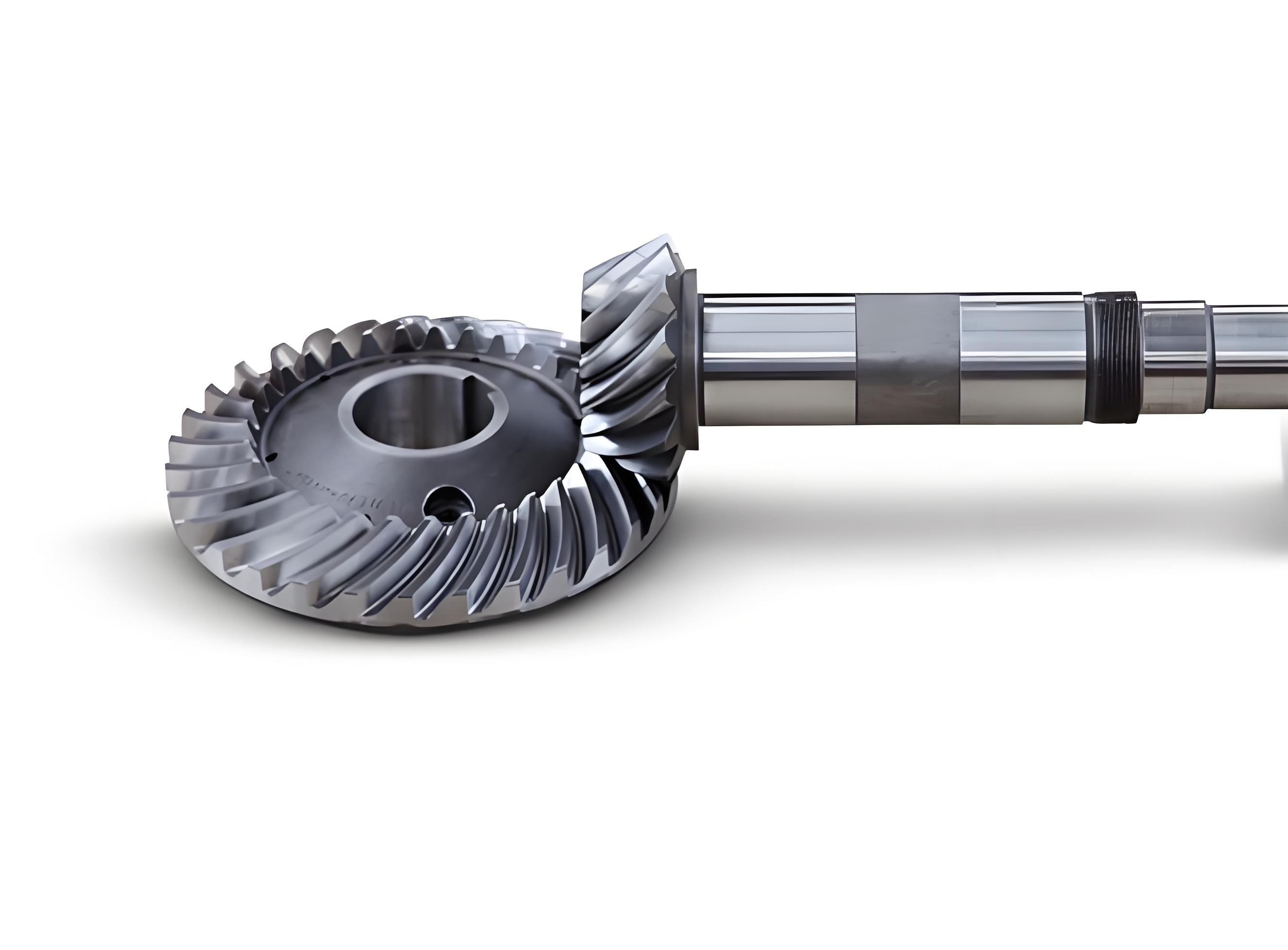
The image above illustrates a typical spiral bevel gear, highlighting its curved teeth that enable smooth engagement. In my modeling approach, such geometry is represented mathematically through the mesh surface, ensuring accuracy in design and analysis. The ability to control the contact region is crucial for optimizing performance in applications like automotive differentials or industrial machinery, where spiral bevel gears are prevalent.
In summary, my method for modeling spiral bevel gears involves creating a mesh surface using tooth trace and spherical involute equations, followed by tooth modification based on local conjugacy principles. This approach simplifies surface representation and modification calculations, making it easier to adjust the contact point position and control the contact region. The parametric nature facilitates automated modeling, reducing manual effort and improving precision. Spiral bevel gears benefit from this method as it ensures reliable performance under varying loads and misalignments. Future work could extend this to other gear types or integrate with advanced manufacturing simulations.
To further elaborate on the advantages, this method reduces the complexity associated with traditional spiral bevel gear design. By using explicit equations, I avoid iterative solutions common in envelope methods. The mesh surface provides a direct way to sample points, which is useful for finite element analysis or CNC programming. Moreover, the modification step is computationally efficient, as it relies on algebraic formulas rather than numerical optimization. This is particularly beneficial for designing spiral bevel gears with customized contact patterns, such as those requiring shifted contact to avoid edge loading or to enhance durability.
Another aspect is the integration with CAD software. By exporting data points to Pro/Engineer, I leverage its robust modeling capabilities to create accurate solids. The motion simulation tools then allow visual inspection of meshing behavior, confirming that the contact region aligns with design intent. For instance, I can simulate scenarios with misalignment or load variations to ensure the spiral bevel gears maintain acceptable contact. This holistic approach from equations to simulation streamlines the design process for spiral bevel gears.
In terms of mathematical depth, the derivation of tooth trace equations involves differential geometry concepts. The invariance of angles on developable surfaces ensures consistency when mapping from the expanded plane to the cone. For spherical involutes, the generation process mimics the rolling of a plane on a base cone, analogous to planar involutes but on a sphere. This geometric foundation ensures that the mesh surface accurately represents the kinematics of spiral bevel gears. I can express key relationships using additional formulas, such as the conversion between spherical and Cartesian coordinates:
Spherical coordinates \( (\rho, \theta, \phi) \) relate to Cartesian coordinates \( (x, y, z) \) by:
$$x = \rho \sin\theta \cos\phi$$
$$y = \rho \sin\theta \sin\phi$$
$$z = \rho \cos\theta$$
Applying this to the tooth trace equation, I obtain points in 3D space for modeling. This coordinate transformation is essential for integrating with CAD systems.
For the modification calculation, the relative curvature formulas derive from the fundamental forms of surfaces. The first fundamental form coefficients \( E, F, G \) and second fundamental form coefficients \( L, M, N \) are used to compute normal curvatures. For a surface defined parametrically, the normal curvature in a direction \( du:dv \) is:
$$k_n = \frac{L du^2 + 2M du dv + N dv^2}{E du^2 + 2F du dv + G dv^2}$$
In the context of spiral bevel gears, these coefficients can be derived from the mesh surface equations, but in practice, I use Gleason’s simplified formulas to expedite the process. This pragmatic approach balances accuracy and efficiency, which is vital for industrial applications involving spiral bevel gears.
To illustrate the computational steps, I outline a procedure in pseudocode:
- Input gear parameters: \( R, \beta, r_0, \theta, \theta_b, l, z_1, r_1, b, f \).
- Generate tooth trace points using equation for \( \rho \) and \( \phi \) over a range of \( \beta’ \).
- Generate spherical involute points using equations for \( x, y, z \) over a range of \( \phi \).
- Combine to form mesh grid: interpolate to get surface points \( P_{ij} \).
- Select contact point \( M \) based on design requirements (e.g., half height, one-third width).
- Calculate modification amounts \( \Delta A \) and \( \Delta B \) using Gleason formulas.
- For each surface point, compute \( \Delta s \) and \( \Delta \delta \) based on relative curvature.
- Adjust point coordinates: \( P’_{ij} = P_{ij} + \Delta \delta \cdot \mathbf{n} \), where \( \mathbf{n} \) is the unit normal.
- Export adjusted points to CAD software for solid modeling.
- Run motion simulation to verify contact region.
This procedure can be implemented in tools like MATLAB or Python, and it highlights the systematic nature of the method. The emphasis on spiral bevel gears throughout ensures clarity in application.
In conclusion, the mesh surface modeling method for spiral bevel gears offers a robust and flexible approach to design. By leveraging parametric equations and local conjugacy-based modification, I achieve precise control over the contact region, which is critical for performance and longevity. The integration with commercial CAD software facilitates practical implementation, making it suitable for engineers designing spiral bevel gears in various industries. As transmission systems evolve, such methods will continue to enhance the reliability and efficiency of spiral bevel gears in demanding applications.