
In this paper, I present a comprehensive study on the multi-objective fuzzy optimization design of cylindrical worm gear drives using Matlab. Worm gears are widely used in various industries such as mining, metallurgy, transportation, and hoisting machinery due to their advantages like large transmission ratio, compact structure, smooth operation, and low noise. However, traditional design methods rely heavily on experience and trial-and-error, often leading to suboptimal solutions. To address the issues of high cost and low efficiency in ordinary cylindrical worm gear drives, I apply fuzzy optimization theory to minimize both the volume of the worm wheel rim and the reciprocal of transmission efficiency. The optimization model is built with carefully chosen design variables, objective functions, and fuzzy constraints. By using Matlab’s optimization toolbox and fuzzy membership functions, a practical and efficient design is obtained.
I first establish the mathematical model for fuzzy optimization. The design variables are chosen as the number of worm gear threads z1, the module m, and the diameter coefficient q. These parameters significantly affect the performance and cost of worm gear drives. The vector of design variables is:
$$X = [x_{1}, x_{2}, x_{3}]^{T} = [z_{1}, m, q]^{T}$$
Two objective functions are considered. The first aims at minimizing the volume of the worm wheel rim, which is made of cast tin bronze and thus costly. The volume is expressed as:
$$f_{1}(X) = \frac{\pi}{4}(d_{e}^{2} – d_{0}^{2})B$$
where:
- de = m(iz1 + 3) is the maximum diameter of the rim,
- d0 = m(iz1 – 6.4) is the minimum diameter,
- B = 0.67m(q + 2) is the width of the rim,
- i = 20 is the transmission ratio.
After substitution and simplification, the first objective function becomes:
$$f_{1}(X) = 0.52622\, x_{2}^{3}(x_{3}+2)\left[(20x_{1}+3)^{2} – (20x_{1}-6.4)^{2}\right]$$
The second objective function is to maximize the transmission efficiency η, which is usually low for worm gears (0.75–0.92). To convert it into a minimization problem, I take the reciprocal of efficiency:
$$f_{2}(X) = \frac{1}{\eta} = \frac{\tan(\lambda + \rho_{v})}{0.96\tan\lambda}$$
where:
- λ = arctan(z1/q) is the lead angle,
- ρv is the equivalent friction angle, with tanρv = fv, the equivalent coefficient of friction.
I use Matlab’s curve fitting to obtain an expression for fv based on standard tables:
$$f_{v} = 0.0175192\, e^{1.0460682 / v_{s}}$$
Here vs is the sliding velocity given by:
$$v_{s} = \frac{m n_{1}}{19100}\sqrt{z_{1}^{2}+q^{2}}$$
With n1 = 960 rpm, the second objective function is expressed in terms of the design variables:
$$f_{2}(X) = \frac{x_{1}x_{3} + f_{v} x_{3}^{2}}{0.96 x_{1} x_{3} – 0.96 x_{1}^{2} f_{v}}$$
Because the two objectives have different magnitudes (the volume is of order 106 mm3 while the efficiency reciprocal is around 1.2), I use a weighted sum method. The weights are chosen as ω1 = 0.8 for volume and ω2 = 0.2 for efficiency reciprocal. To balance the order, f2 is multiplied by 106. The unified objective function is:
$$f(X) = 0.8 f_{1}(X) + 0.2 \times 10^{6} f_{2}(X)$$
$$f(X) = 0.420976\, x_{2}^{3}(x_{3}+2)\left[(20x_{1}+3)^{2} – (20x_{1}-6.4)^{2}\right] – \frac{4.8\times10^{6}(x_{1}x_{3}+f_{v}x_{3}^{2})}{x_{1}(x_{3}-x_{1}f_{v})}$$
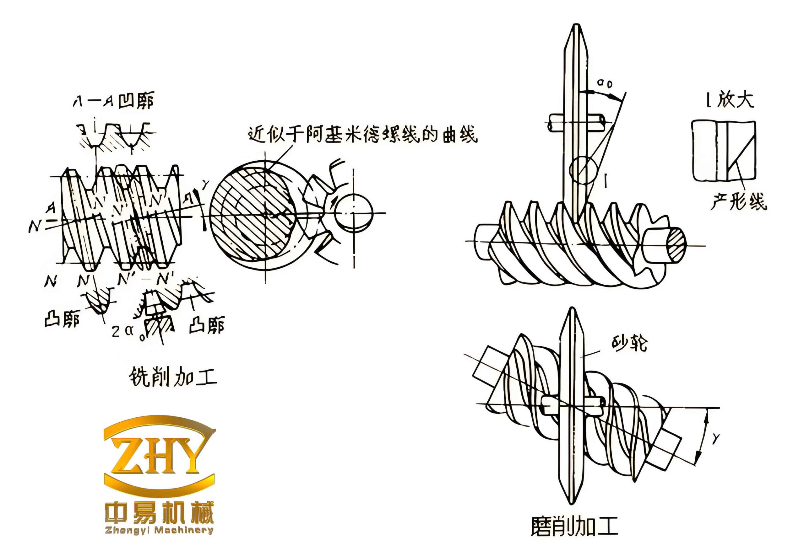
Next, I construct the constraint conditions. Both geometric and performance constraints typically exhibit fuzziness, with a transition zone from fully allowable to completely disallowable. The constraints are as follows.
Boundary Constraints
| Variable | Lower bound | Upper bound | Expression |
|---|---|---|---|
| Number of worm threads z1 | 2 | 6 | 2 ≤ g1(X) = x1 ≤ 6 |
| Number of worm wheel teeth z2 = 20z1 | 30 | 80 | 30 ≤ g2(X) = 20x1 ≤ 80 |
| Module m (mm) | 2 | 18 | 2 ≤ g3(X) = x2 ≤ 18 |
| Diameter coefficient q | 8 | 15 | 8 ≤ g4(X) = x3 ≤ 15 |
Performance Constraints
- Contact fatigue strength of worm wheel teeth
$$\sigma_{H} = Z_{E} \sqrt{\frac{9400\,T_{2}\,K_{A}\,K_{V}\,K_{\beta}}{d_{1}d_{2}^{2}}} \leq [\sigma_{H}]$$
With material coefficient ZE = 155 √MPa, torque T2 = 1.26836×10⁶ N·mm, d1= mq, d2 = miz1, and coefficients KA=1.0, KV=1.1, Kβ=1.0. The allowable stress [σH] = 166.57 MPa. After simplification:
$$g_{5}(X) = \frac{28066.176}{\sqrt{x_{1}^{2} x_{2}^{3} x_{3}}} \leq [\sigma_{H}]$$
- Bending fatigue strength of worm wheel teeth
$$\sigma_{F} = \frac{666\,T_{2}\,K_{A}\,K_{V}\,K_{\beta}}{d_{1}d_{2}m}\,Y_{Fs}\,Y_{\beta} \leq [\sigma_{F}]$$
The composite tooth factor YFs is fitted as YFs = 2.58 e–0.049z1, and the lead angle factor Yβ = 1 – λ/120°. The allowable stress [σF] = 38.164 MPa. Thus:
$$g_{6}(X) = \frac{119866.869\, e^{-0.049 x_{1}} \left(1 – \frac{\arctan(x_{1}/x_{3})}{120}\right)}{x_{1} x_{2}^{3} x_{3}} \leq [\sigma_{F}]$$
- Worm shaft deflection
The deflection f at the meshing point must satisfy:
$$f = \frac{\sqrt{F_{r1}^{2}+F_{t1}^{2}}}{48EI}L^{3} \leq [f]$$
After derivation with Ft1 = 2T2/(iηmq), Fr1 = 2T2 tan20°/(miz1), I = πm4(q–2.4)4/64, L = 1.1m(iz1+2), and [f] = m/50, the constraint becomes:
$$g_{7}(X) = \frac{3.411852\times10^{-4}\,(20x_{1}+2)^{3}\sqrt{\left(\frac{0.36397}{x_{1}}\right)^{2}+\left(\frac{1.17647}{x_{3}}\right)^{2}}}{(x_{3}-2.4)^{4}x_{2}^{2}} \leq \frac{x_{2}}{50}$$
- Sliding velocity
$$v_{s} = \frac{m n_{1}}{19100}\sqrt{z_{1}^{2}+q^{2}} \leq [v_{s}] = 16\ \text{m/s}$$
Hence:
$$g_{8}(X) = 0.05026178\, x_{2} \sqrt{x_{1}^{2}+x_{3}^{2}} \leq 16$$
- Thermal balance condition
The temperature rise Δt must be within 60 °C:
$$\Delta t = \frac{1000P(1-\eta)}{k_{s} A} \leq [\Delta t]$$
With P = 7.5 kW, η estimated as 0.85, ks = 15 W/(m2·°C), and A = 0.33(a/100)1.75 where a = m(q+iz1)/2. After simplification:
$$g_{9}(X) = \frac{2417407.226}{\left[x_{2}(x_{3}+20x_{1})\right]^{1.75}} \leq 60$$
To handle fuzzy constraints, I define linear membership functions for both performance and boundary constraints. The transition intervals are determined by the expansion coefficient method. For upper bounds, the expansion coefficient β+ is taken as 1.05, and for lower bounds, β– = 0.85. The resulting fuzzy allowable intervals are listed in the table below.
| Constraint | Upper bound – upper limit | Upper bound – lower limit | Lower bound – upper limit | Lower bound – lower limit |
|---|---|---|---|---|
| [σH] (MPa) | 174.9 | 166.6 | – | – |
| [σF] (MPa) | 40.07 | 38.16 | – | – |
| [f] (mm) | 0.021m | 0.02m | – | – |
| [vs] (m/s) | 16.8 | 16 | – | – |
| [Δt] (°C) | 63 | 60 | – | – |
| z1 | 6.3 | 6 | 2 | 1.7 |
| m (mm) | 18.9 | 18 | 2 | 1.7 |
| q | 15.75 | 15 | 8 | 6.8 |
| z2 (20z1) | 84 | 80 | 30 | 25.5 |
The optimal level cut λ* is determined by fuzzy comprehensive evaluation. After constructing the factor set, evaluation set, and weight set, and applying the fuzzy operator M(·,⊕), I obtain λ* = 0.6. This level cut transforms the fuzzy optimization into a deterministic non-fuzzy problem. The constraints become:
- 1.88 ≤ x1 ≤ 6.12
- 28.2 ≤ 20x1 ≤ 81.6
- 1.88 ≤ x2 ≤ 18.36
- 7.52 ≤ x3 ≤ 15.35
- g5(X) ≤ 169.92
- g6(X) ≤ 38.924
- g7(X) ≤ 0.0204 x2
- g8(X) ≤ 16.32
- g9(X) ≤ 61.2
I then implement the optimization in Matlab. The objective function is defined in the M-file `myobj.m`:
function f = myobj(x)
    f = 0.420976 * x(2)^3 * (x(3)+2) * ((20*x(1)+3)^2 - (20*x(1)-6.4)^2) ...
        - (4.8e6 * (x(1)*x(3) + 0.0175192*exp(1.0460682/(0.05026178*x(2)*sqrt(x(1)^2+x(3)^2))) * x(3)^2)) ...
          / (x(1)*(x(3) - x(1)*0.0175192*exp(1.0460682/(0.05026178*x(2)*sqrt(x(1)^2+x(3)^2)))));
end
The nonlinear constraints are written in `mycon.m`:
function [c, ceq] = mycon(x)
    c(1) = 28066.176 / sqrt(x(1)^2 * x(2)^3 * x(3)) - 169.92;
    c(2) = 119866.869 * exp(-0.049*x(1)) * (1 - atan(x(1)/x(3))/120) / (x(1)*x(2)^3*x(3)) - 38.924;
    c(3) = 3.411852e-4 * (20*x(1)+2)^3 * sqrt((0.36397/x(1))^2 + (1.17647/x(3))^2) / ((x(3)-2.4)^4 * x(2)^2) - 0.0204*x(2);
    c(4) = 0.05026178 * x(2) * sqrt(x(1)^2 + x(3)^2) - 16.32;
    c(5) = 2417407.226 / (x(2)*(x(3)+20*x(1)))^1.75 - 61.2;
    ceq = [];
end
The bounds and linear constraints are set, and the `fmincon` solver is called:
lb = [1.7, 1.7, 6.8];
ub = [6.3, 18.9, 15.75];
x0 = [1.7, 1.7, 6.8];
A = [-1,0,0; 1,0,0; 0,-1,0; 0,1,0; 0,0,-1; 0,0,1];
b = [-1.88, 4.08, -1.88, 18.36, -7.52, 15.35];
options = optimset('display','off','largescale','off');
[x, fval] = fmincon(@myobj, x0, A, b, [], [], lb, ub, @mycon, options);
The optimal solution obtained is X = [4.08, 4.743, 15.35]. After rounding to standard values: z1 = 4, m = 5 mm, q = 15. The results are compared with the traditional design (z1 = 2, m = 8 mm, q = 10) in the table below.
| Parameter | Traditional | Optimized |
|---|---|---|
| z1 | 2 | 4 |
| m (mm) | 8 | 5 |
| q | 10 | 15 |
| Worm wheel rim volume V (mm3) | 2.327958 × 10⁶ | 1.64606 × 10⁶ |
| Transmission efficiency η | 0.8586 | 0.8787 |
| Volume reduction (%) | – | 29.3% |
| Efficiency improvement (%) | – | 2.34% |
The optimized design for these worm gears achieves a 29.3% reduction in wheel rim volume while improving the transmission efficiency by 2.34%. This demonstrates the effectiveness of the multi-objective fuzzy optimization approach. The use of Matlab simplifies the computation and makes the method readily applicable to engineering practice. The methodology can be extended to other types of worm gears and similar mechanical drives where conflicting objectives and fuzzy constraints exist.
In conclusion, this paper provides a systematic procedure for optimizing cylindrical worm gear drives using fuzzy set theory and Matlab. By considering both cost (volume) and performance (efficiency) with appropriate fuzzy constraints, the design becomes more rational and yields significant improvements. Engineers can adopt this approach to design high-quality worm gears with reduced material consumption and enhanced operational efficiency.