
In recent years, with the increasing global energy crisis and environmental concerns, green and low-energy manufacturing technologies have gained significant attention. Compared to traditional wet cutting, high-speed dry gear hobbing represents a major innovation due to its eco-friendly and efficient characteristics. This process is widely used in gear manufacturing. However, due to the high cutting speeds and absence of cutting fluid for cooling and lubrication, substantial heat is generated per unit time. Inappropriate process parameters can severely affect gear quality errors, tool life, and energy utilization of the gear hobbing machine. Therefore, it is essential to comprehensively consider multiple objectives such as energy consumption, tool life, and quality error to conduct research on process parameter optimization, achieving overall optimal machining performance.
Currently, numerous studies have been conducted on the optimization of gear hobbing process parameters. These studies primarily focus on single or dual objective optimization models based on energy consumption, tool life, machining cost, etc., using intelligent algorithms and experimental research for parameter optimization. However, there are still shortcomings: in high-speed dry gear hobbing, when optimizing energy consumption, if only the cutting stage is considered, energy may not be utilized to its fullest extent; research on multi-objective optimization for three or more objectives in high-speed dry gear hobbing is relatively scarce; and when solving multi-objective optimization models with optimization algorithms, after obtaining the solution set of process parameters, selection often relies on empirical knowledge without ranking the solutions for better decision-making efficiency.
With the development of clean cutting technology, higher requirements are placed on the energy utilization of high-speed dry gear hobbing machines. Simultaneously, during high-speed cutting, significant heat leads to severe tool wear, reducing tool life and affecting cutting performance. The application of gears with high rotational speed, high efficiency, and low noise also imposes stringent demands on the quality of high-speed dry gear hobbing. Single or dual objective models can no longer adequately meet machining needs. It is necessary to comprehensively consider total energy consumption across machine stages, tool life, gear workpiece quality, and other objectives to conduct process parameter optimization research and rank the solution set for improved decision-making efficiency, which is an inevitable direction for the future development of high-speed dry gear hobbing.
To address these issues, we establish a multi-objective optimization model with the goals of minimum energy consumption, minimum quality error, and maximum tool life. We employ the NSGA-III algorithm based on reference points for iterative optimization to obtain an optimized set of process parameters. Then, we use the AHP-TOPSIS combined method, where AHP calculates the weights of each evaluation indicator, and TOPSIS completes the ranking of the solution set. This approach facilitates more efficient and reasonable optimization decisions.
Problem Description
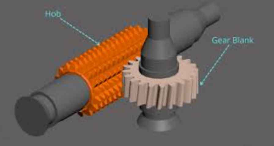
The factors influencing the characteristics of high-speed dry gear hobbing are numerous, primarily including workpiece parameters, hob performance parameters, and machine parameters. These parameters have complex relationships and affect the optimization objectives differently. In the context of green manufacturing, optimizing energy consumption is particularly important. The application of gears with high rotational speed, high efficiency, and low noise also requires higher quality in gear hobbing. During high-speed dry gear hobbing, tool life is severely affected by the substantial heat generated per unit time. To achieve comprehensive optimization of machining characteristics, it is necessary to study the relationships between energy consumption, hob life, quality error, and process parameters, and establish an effective multi-objective optimization model.
We formulate the gear hobbing process problem as follows:
Let \( G = \{ G_1, G_2, G_3, \ldots, G_n \} \), where \( G_i \) represents the \( i \)-th set of process parameters, defined as \( G_i = \{ gp_i, tp_i, pp_i \} \). Here, \( gp_i \) denotes workpiece parameters, \( tp_i \) denotes tool performance parameters, and \( pp_i \) denotes hobbing process parameters.
Thus, for a given gear hobbing task, the process variable problem can be expressed as:
Workpiece parameters: \( gp = ( m_n, z_1, \alpha, \beta, d_{a1}, B ) \), where \( m_n \) is the normal module, \( z_1 \) is the number of teeth on the gear, \( \alpha \) is the pressure angle, \( \beta \) is the helix angle, \( d_{a1} \) is the outer diameter of the gear, and \( B \) is the face width.
The process parameters that need optimization are represented as \( \{ tp, pp \} = \{ ( z_2, d_{a2}, n_i ), ( f_z, n_z, a_p ) \} \), where \( z_2 \) is the number of hob threads, \( d_{a2} \) is the hob diameter, \( n_i \) is the gear ratio, \( f_z \) is the axial feed per revolution, \( n_z \) is the spindle speed, and \( a_p \) is the cutting depth. Each variable’s attributes are illustrated in the following table:
| Parameter Type | Symbol | Description |
|---|---|---|
| Workpiece Parameters | \( m_n \) | Normal module |
| \( z_1 \) | Number of gear teeth | |
| \( \alpha \) | Pressure angle | |
| \( \beta \) | Helix angle | |
| \( d_{a1} \) | Gear outer diameter | |
| \( B \) | Face width | |
| Tool Parameters | \( z_2 \) | Number of hob threads |
| \( d_{a2} \) | Hob diameter | |
| \( n_i \) | Gear ratio | |
| Process Parameters | \( f_z \) | Axial feed per revolution |
| \( n_z \) | Spindle speed | |
| \( a_p \) | Cutting depth |
The variables to be optimized significantly influence energy consumption, quality error, and tool life during gear hobbing. Therefore, coordinating these parameters is a key issue. In actual gear hobbing processes, the cutting depth \( a_p \) has minimal impact on the gear hobbing machine and workpiece, so it is not considered in the optimization. Among the cutting parameters, axial feed and spindle speed are critical. Additionally, hob performance parameters, particularly hob diameter \( d_{a2} \) and number of threads \( z_2 \), cannot be ignored. Thus, the number of hob grooves is not a decision variable. Based on analysis of influential factors in gear hobbing, we select the most important parameters as decision variables for optimization: \( \{ f_z, n_z, d_{a2}, z_2 \} \).
Multi-objective Optimization Model
We analyze the energy consumption at various stages of the gear hobbing process and use mathematical functions to characterize tool life and quality error after gear hobbing. A multi-objective optimization model is constructed with the goals of minimizing energy consumption, minimizing quality error, and maximizing tool life.
Energy Consumption Model
Energy consumption in a gear hobbing machine during operation takes various forms and follows complex patterns. From machine startup to completion, energy consumption differs at each stage. Considering the factors contributing to energy consumption at each stage, the energy consumption can be converted into power and time consumption.
The startup process of the gear hobbing machine, which involves activating basic components like the lighting system, is very brief and consumes negligible energy, so it is ignored in the model.
After startup, the machine enters standby mode, where basic components operate steadily. The power during this stage is determined solely by the machine’s performance parameters and is independent of external factors. This power can be directly measured. The energy consumption during standby is:
$$ E_{\text{standby}} = P_{\text{standby}} T_{\text{standby}} $$
During gear hobbing, there is an idle cutting phase where the tool does not engage with the workpiece. Energy consumption in this phase mainly comes from the stable operation of the spindle motor, servo motors, and other machine components and auxiliary systems. The energy consumption for idle cutting is:
$$ E_{\text{empty}} = P_{\text{empty}} T_{\text{empty}} $$
\( P_{\text{empty}} \) consists of standby power, auxiliary system power, and no-load power consumption of the motors:
$$ P_{\text{empty}} = P_{\text{standby}} + P_{\text{assist}} + P_{\text{emotor}} $$
where \( P_{\text{assist}} \) is the power consumed by auxiliary systems such as cooling, lubrication, loading/unloading, and lighting.
Based on fitting experimental data and research, the total power consumption of the motors has a quadratic relationship with spindle speed. Thus, the no-load power consumption of the motors \( P_{\text{emotor}} \) is expressed as:
$$ P_{\text{emotor}} = a_1 n_z^2 + b_1 n_z + c_1 $$
where \( n_z \) is the spindle speed, and coefficients \( a_1 \), \( b_1 \), \( c_1 \) are related to the power characteristics of the gear hobbing machine motors.
The idle travel consists of tool paths in the X-axis (radial) and Z-axis (axial) directions. The time for this process is denoted as idle cutting time \( T_{\text{empty}} \):
$$ T_{\text{empty}} = \sum_{n_{\text{walk}}} \frac{S_x}{F_x} + \sum_{n_{\text{walk}}} \frac{S_z}{F_z} $$
where \( n_{\text{walk}} \) is the number of tool passes, \( S_x \) is the radial travel distance, \( F_x \) is the radial feed rate, \( S_z \) is the axial travel distance, and \( F_z \) is the axial feed rate.
The cutting phase involves material removal from the workpiece. The total power consumption during cutting includes standby power, auxiliary system power, motor no-load power, cutting power, and power losses due to load. The cutting force \( F_{\text{cut}} \) is given by:
$$ F_{\text{cut}} = \frac{c_f k_1 k_2 k_3 m_t^{x_f} f_z^{y_f} a_p^{z_f} v_{\text{cut}}^{-u_f} z_1^{v_f}}{d_{a2}} $$
where \( c_f \), \( x_f \), \( y_f \), \( z_f \), \( u_f \), \( v_f \) are coefficients related to cutting force; \( k_1 \), \( k_2 \), \( k_3 \) are workpiece-related coefficients; and \( m_t \) is the tool normal module.
The cutting speed \( v_{\text{cut}} \) is:
$$ v_{\text{cut}} = \frac{\pi d_{a2} n_z}{1000} $$
Research indicates that the power loss due to load \( P_{\text{load}} \) has a quadratic relationship with cutting power \( P_{\text{cut}} \):
$$ P_{\text{load}} = a_2 P_{\text{cut}}^2 + b_2 P_{\text{cut}} + c_2 $$
The cutting time \( T_{\text{cut}} \) can be calculated from the cutting travel and axial feed rate:
$$ T_{\text{cut}} = \frac{S_{\text{cut}}}{F_z} $$
where \( S_{\text{cut}} \) is the cutting travel distance, expressed as:
$$ S_{\text{cut}} = \left[ (d_{a2} + d_{a1}) \tan^2 \delta + d_{a2} \right] a_p + 1.25 m_n \sin \delta / \tan \alpha + B + E + U $$
Here, \( \delta \) is the setting angle, \( E \) and \( U \) are safe approach and exit distances during gear hobbing, and \( \alpha \) is the pressure angle.
The axial feed rate \( F_z \) is related to hob threads and spindle speed:
$$ F_z = \frac{z_2 f_z n_z}{z_1} $$
The total energy consumption during the cutting phase \( E^{\text{total}}_{\text{cut}} \) is:
$$ E^{\text{total}}_{\text{cut}} = (P_{\text{empty}} + P_{\text{cut}} + P_{\text{load}}) T_{\text{cut}} $$
Thus, the total energy consumption for gear hobbing is:
$$ E_{\text{total}} = E_{\text{standby}} + E_{\text{empty}} + E^{\text{total}}_{\text{cut}} $$
Tool Life Model
In high-speed dry gear hobbing, tool wear and breakage are common, affecting machining quality and overall performance. To extend tool life, appropriate process parameters must be selected. Tool life can be measured in various ways, such as the number of workpieces machined, machining time, or total workpieces machined until tool failure. However, each method has limitations. We express tool life \( L_{\text{tool}} \) as:
$$ L_{\text{tool}} = \frac{C_v}{v_{\text{cut}} f_z^{y_v} m_t^{x_v} K_v^{m_v – 1}} $$
where \( C_v \), \( K_v \), \( x_v \), \( y_v \), \( m_v \) are tool-related coefficients.
Quality Error Model
The final quality in gear hobbing is influenced by multiple factors related to tool, workpiece, and cutting parameters. During gear hobbing, the tool may produce equidistant jumps per axial feed \( f_z \), and misalignment between the machine tool’s vertical feed direction and the workpiece axis can cause deviations along the tooth trace. In practice, gears cannot have perfect involute tooth profiles, leading to tooth profile errors. To evaluate gear quality comprehensively, we introduce a weighted model for quality error. The tooth trace error \( e_x \) and tooth profile error \( e_y \) are given by:
$$ e_x = \frac{f_z^2 \sin \alpha}{4 d_{a2} \cos^2 \beta} $$
$$ e_y = \frac{(\pi z_2)^2 m_n \sin \alpha}{4 z_1 n_i^2} $$
Considering both errors equally, we assign weights of 0.5 each. The quality error model \( Q_{\text{error}} \) is:
$$ Q_{\text{error}} = 0.5 e_x + 0.5 e_y $$
Optimization Model and Constraints
Based on the above analysis, we establish a multi-objective optimization model to minimize energy consumption, minimize quality error, and maximize tool life. The optimization function is:
$$ f = (\min E_{\text{total}}, \min Q_{\text{error}}, \max L_{\text{tool}}) $$
In actual gear hobbing, parameter optimization is subject to various constraints, including machine performance, quality requirements, and hob specifications. The decision variables must satisfy the following constraints:
- \( n_{\min} \leq n_z \leq n_{\max} \): Spindle speed must be within the machine’s allowable range.
- \( (f_z)_{\min} \leq f_z \leq (f_z)_{\max} \): Axial feed per revolution must be within the machine’s allowable range.
- \( F_{\text{cut}} \leq (F_{\text{cut}})_{\max} \): Cutting force must not exceed the machine’s maximum cutting force.
- \( R_a = 0.312 \frac{f_z^2}{r} \leq [R_a] \): Surface roughness of the gear after machining must be within the maximum roughness limit, where \( r \) is the hob radius.
Optimization and Decision-making Method
NSGA-III Algorithm for Optimization
When solving multi-objective optimization problems, traditional algorithms often convert them into single-objective problems by introducing weights. However, these algorithms may impose idealized conditions that deviate from reality, leading to suboptimal solutions. With the development of intelligent optimization algorithms, many methods suitable for multi-objective problems have emerged, providing better solutions.
NSGA-III (Non-dominated Sorting Genetic Algorithm III) was proposed in 2014. Its solution approach is similar to NSGA-II, but the main difference lies in the selection operator. NSGA-III uses a reference-point-based strategy for individual selection instead of crowding distance. This improves algorithm convergence and solution set uniformity, especially for problems with three or more objectives. The main flowchart of the NSGA-III algorithm is as follows:
Step 1: Generate reference points \( H \) based on the number of optimization objectives \( M \) and decision variables \( n_{\text{var}} \).
Step 2: For the \( t \)-th generation population \( P_t \), generate offspring population \( Q_t \) through crossover and mutation. The population size for each generation is \( N \). Combine parent \( P_t \) and offspring \( Q_t \) to form population \( R_t \) with size \( 2N \).
Step 3: Perform non-dominated sorting on \( R_t \) to obtain several non-dominated fronts \( F_1, F_2, \ldots, F_i \).
Step 4: Store higher-priority non-dominated fronts in archive set \( S_t \). Assume the critical front is \( F_l \).
Step 5: Based on the reference points generated in Step 1, connect each reference point to the origin to form reference vectors. Calculate the perpendicular distance from each individual in \( S_t \) to the reference vectors and associate each individual with the closest reference vector.
Step 6: Select individuals from \( F_l \) to form population \( P_{t+1} \) of size \( N \) using the closest distance principle. Filter this population to obtain the next generation \( P_{t+1} \). If the iteration count exceeds the maximum \( K_{\max} \), output the final population as the optimized process parameter solution set; otherwise, return to Step 2.
For the multi-objective optimization of high-speed dry gear hobbing process parameters, the NSGA-III steps are applied accordingly.
AHP-TOPSIS Combined Method for Ranking
AHP (Analytic Hierarchy Process) is a method for quantitative analysis of qualitative problems. TOPSIS (Technique for Order Preference by Similarity to Ideal Solution) ranks alternatives based on their closeness to an ideal solution. We combine the advantages of AHP and TOPSIS in an AHP-TOPSIS method to rank the process parameter solution set. The framework is as follows:
- Let \( m \) be the number of evaluation indicators. Construct a pairwise comparison matrix \( A \) for the indicators:
$$ A = \begin{bmatrix} 1 & a_{12} & \cdots & a_{1n} \\ a_{21} & 1 & \cdots & a_{2n} \\ \vdots & \vdots & \ddots & \vdots \\ a_{n1} & a_{n2} & \cdots & 1 \end{bmatrix} $$
where \( a_{ij} \) represents the importance of the \( i \)-th indicator relative to the \( j \)-th indicator. - Let \( n \) be the number of process parameter solutions. Form the original data matrix \( X \):
$$ X = \begin{bmatrix} x_{11} & x_{12} & \cdots & x_{1m} \\ x_{21} & x_{22} & \cdots & x_{2m} \\ \vdots & \vdots & \ddots & \vdots \\ x_{n1} & x_{n2} & \cdots & x_{nm} \end{bmatrix} $$
where \( x_{ij} \) is the raw value of the \( j \)-th evaluation indicator for the \( i \)-th solution. - Normalize matrix \( X \) to obtain matrix \( G \):
$$ G = \begin{bmatrix} x’_{11} & x’_{12} & \cdots & x’_{1m} \\ x’_{21} & x’_{22} & \cdots & x’_{2m} \\ \vdots & \vdots & \ddots & \vdots \\ x’_{n1} & x’_{n2} & \cdots & x’_{nm} \end{bmatrix} $$
where \( x’_{ij} = \frac{x_{ij}}{\sqrt{\sum_{k=1}^{n} x_{kj}^2}} \), for \( i = 1,2,\ldots,n \) and \( j = 1,2,\ldots,m \). - Apply weights to form the weighted normalized matrix \( Z \):
$$ Z = \begin{bmatrix} z_{11} & z_{12} & \cdots & z_{1m} \\ z_{21} & z_{22} & \cdots & z_{2m} \\ \vdots & \vdots & \ddots & \vdots \\ z_{n1} & z_{n2} & \cdots & z_{nm} \end{bmatrix} $$
where \( z_{ij} = x’_{ij} \times \varepsilon_j \), and \( \varepsilon_j \) is the weight of the \( j \)-th indicator calculated by AHP. - Determine the ideal best \( Z^+ \) and ideal worst \( Z^- \) solutions:
$$ Z^+ = (z^+_1, z^+_2, \ldots, z^+_m) $$
$$ Z^- = (z^-_1, z^-_2, \ldots, z^-_m) $$
where \( z^+_j = \max(z_{ij}) \) for benefit criteria or \( \min(z_{ij}) \) for cost criteria, and \( z^-_j = \min(z_{ij}) \) for benefit criteria or \( \max(z_{ij}) \) for cost criteria. - Calculate the Euclidean distances from each solution to \( Z^+ \) and \( Z^- \):
$$ S^+_i = \sqrt{\sum_{j=1}^{m} (z_{ij} – z^+_j)^2} $$
$$ S^-_i = \sqrt{\sum_{j=1}^{m} (z_{ij} – z^-_j)^2} $$ - Compute the relative closeness \( C_i \) to the ideal solution:
$$ C_i = \frac{S^-_i}{S^+_i + S^-_i} $$
\( C_i \) ranges from 0 to 1, with higher values indicating better performance.
Experimental Verification
We conduct gear hobbing experiments on a YDZ3126CNC machine. The machine performance parameters are listed in the following table:
| Parameter | Value |
|---|---|
| Spindle Speed \( n_z \) | 0–2500 rpm |
| Radial Feed Rate \( F_x \) | 0–7500 mm/min |
| Axial Feed Rate \( F_z \) | 0–7500 mm/min |
| Maximum Module | 6 mm |
| Tangential Stroke | 0–200 mm |
| Maximum Diameter | 260 mm |
The gear workpiece parameters are:
| Parameter | Value |
|---|---|
| Material | 45 Steel |
| Module \( m_n \) | 2.5 mm |
| Number of Teeth \( z_1 \) | 51 |
| Pressure Angle \( \alpha \) | 20° |
| Helix Angle \( \beta \) | 19° |
| Outer Diameter \( d_{a1} \) | 132.5 mm |
| Face Width \( B \) | 45 mm |
The hob performance parameters are:
| Parameter | Value |
|---|---|
| Material | High-Speed Steel |
| Normal Module \( m_t \) | 2 mm |
| Number of Grooves | 12 |
| Setting Angle | 18° |
| Helix Angle | 3.16° |
| Hand | Right-hand |
The coefficients for energy consumption calculation are:
| Parameter | Value |
|---|---|
| \( P_{\text{standby}} \) | 2300 W |
| \( P_{\text{assist}} \) | 245 W |
| \( T_{\text{standby}} \) | 3.5 min |
| \( a_1 \) | 2.13 × 10⁻⁶ |
| \( a_2 \) | 1.33 × 10⁻⁵ |
| \( b_1 \) | -0.08 |
| \( b_2 \) | 0.035 |
| \( c_1 = c_2 \) | 0 |
The parameters for cutting process calculation are:
| Parameter | Value |
|---|---|
| \( S_x \) | 110.6 mm |
| \( S_z \) | 22.15 mm |
| \( F_x \) | 1500 mm/min |
| \( a_p \) | 6.5 mm |
| \( E \) | 2 mm |
| \( U \) | 2 mm |
The coefficients for cutting force and tool life are:
| Coefficient | Value |
|---|---|
| \( c_f \) | 18.2 |
| \( u_f \) | 0.27 |
| \( v_f \) | 0.28 |
| \( x_f \) | 1.76 |
| \( y_f \) | 0.65 |
| \( z_f \) | 0.82 |
| \( k_1 \) | 1 |
| \( k_2 \) | 1.08 |
| \( k_3 \) | 1.11 |
| \( C_v \) | 289 |
| \( K_v \) | 0.68 |
| \( x_v \) | 0 |
| \( y_v \) | 0.5 |
| \( m_v \) | 0.33 |
We implement the NSGA-III algorithm in MATLAB. The number of reference points is set to 15, population size \( N = 100 \), and maximum iterations \( K_{\max} = 800 \). Based on actual machining conditions, the decision variable ranges are:
$$ 1.2 \leq f_z \leq 2 \text{ mm/rev} $$
$$ 700 \leq n_z \leq 1300 \text{ rpm} $$
$$ 75 \leq d_{a2} \leq 90 \text{ mm}, \quad d_{a2} \in \mathbb{N} $$
$$ 1.9 \leq z_2 \leq 3.1, \quad z_2 \in \mathbb{N} $$
The NSGA-III algorithm yields a Pareto solution set distributed in the objective space. The optimized process parameter solution set includes 30 solutions. A subset of these solutions is shown in the following table:
| Solution \( J_i \) | \( f_z \) (mm/rev) | \( n_z \) (rpm) | \( d_{a2} \) (mm) | \( z_2 \) (integer) | \( Q_{\text{error}} \) (mm) | \( E_{\text{total}} \) (J) | \( L_{\text{tool}} \) (min) |
|---|---|---|---|---|---|---|---|
| J1 | 1.5516 | 1300 | 90 | 3 | 0.0286 | 6,632,490 | 330.3415 |
| J2 | 1.3510 | 1300 | 90 | 3 | 0.0229 | 7,148,332 | 330.1892 |
| J3 | 1.2814 | 1265.4 | 84 | 2 | 0.0205 | 7,769,636 | 330.1508 |
| J4 | 1.4497 | 1300 | 89 | 3 | 0.0245 | 6,941,909 | 330.1884 |
| J5 | 1.2988 | 1267.2 | 98 | 3 | 0.0217 | 7,588,220 | 330.2103 |
| … | … | … | … | … | … | … | … |
| J30 | 1.3918 | 1276.3 | 89 | 3 | 0.0237 | 7,220,303 | 330.1503 |
To analyze the relationships between cutting parameters and optimization objectives, we plot \( f_z \) and \( n_z \) against each objective. The plots show that changing any decision variable affects the objectives in different directions, highlighting the need for comprehensive consideration when selecting parameters.
Since the NSGA-III algorithm operates on continuous variables, but some parameters like hob threads are discrete, the solution set may have variations in quality. To facilitate efficient decision-making, we apply the AHP-TOPSIS method to rank the solutions.
We use energy consumption, quality error, and tool life as evaluation indicators. In AHP, we assign weights based on relative importance: energy consumption is prioritized over quality error, and quality error over tool life. The calculated weights are: \( \varepsilon_E = 0.5396 \) for energy consumption, \( \varepsilon_Q = 0.2970 \) for quality error, and \( \varepsilon_L = 0.1634 \) for tool life.
Using TOPSIS, we compute the relative closeness \( C_i \) for each solution. The top 15 ranked solutions are:
| Solution | Relative Closeness \( C_i \) | Rank |
|---|---|---|
| J2 | 0.72839 | 1 |
| J21 | 0.70731 | 2 |
| J10 | 0.70436 | 3 |
| J4 | 0.69739 | 4 |
| J25 | 0.69606 | 5 |
| J29 | 0.69119 | 6 |
| J9 | 0.67658 | 7 |
| J30 | 0.66815 | 8 |
| J12 | 0.66774 | 9 |
| J13 | 0.65457 | 10 |
| J8 | 0.64959 | 11 |
| J15 | 0.64681 | 12 |
| J6 | 0.64136 | 13 |
| J7 | 0.64073 | 14 |
| J11 | 0.63562 | 15 |
The highest-ranked solution is J2, with parameters \( \{ f_z = 1.3510 \text{ mm/rev}, n_z = 1300 \text{ rpm}, d_{a2} = 90 \text{ mm}, z_2 = 3 \} \). This solution is recommended when considering all three objectives comprehensively. If minimizing energy consumption is the primary goal, J1 is preferred; for minimizing quality error, J3 is best; and for maximizing tool life, J7 is optimal.
To validate the effectiveness of our method, we compare it with other popular optimization algorithms: NSGA-II and MOPSO (Multi-Objective Particle Swarm Optimization). The Pareto solution sets from NSGA-II and MOPSO are more dispersed in the objective space, whereas NSGA-III produces a more concentrated set. Using AHP-TOPSIS on the solutions from all algorithms, we compare the best solutions. The results are summarized in the following table:
| Method | \( f_z \) (mm/rev) | \( n_z \) (rpm) | \( d_{a2} \) (mm) | \( z_2 \) | \( E_{\text{total}} \) (J) | \( Q_{\text{error}} \) (mm) | \( L_{\text{tool}} \) (min) |
|---|---|---|---|---|---|---|---|
| Our Method (NSGA-III + AHP-TOPSIS) | 1.3510 | 1300 | 90 | 3 | 7,148,332 | 0.0229 | 330.1892 |
| NSGA-II | 1.3813 | 1293.7 | 89 | 3 | 7,267,248 | 0.0240 | 330.1020 |
| MOPSO | 1.6348 | 1289 | 89 | 2 | 7,462,018 | 0.0245 | 330.1180 |
Compared to NSGA-II, our method reduces energy consumption by 1.64%, decreases quality error by 4.58%, and increases tool life by 0.026%. Compared to MOPSO, it reduces energy consumption by 4.2%, decreases quality error by 6.53%, and increases tool life by 0.022%. These results demonstrate the effectiveness of our approach.
Conclusion
To achieve comprehensive optimization of energy consumption, tool life, and workpiece quality in high-speed dry gear hobbing, we established a multi-objective optimization model with axial feed, hob diameter and threads, and spindle speed as decision variables, and minimum energy consumption, minimum quality error, and maximum tool life as objectives. Leveraging the advantages of the reference-point-based NSGA-III algorithm for problems with three or more objectives, we solved the model and obtained a Pareto solution set uniformly distributed in the objective space. Using the AHP-TOPSIS combined method, we calculated the weights of energy consumption, quality error, and tool life via AHP and ranked the solution set via TOPSIS, providing an intuitive ranking of process parameter schemes and improving decision-making efficiency. Based on cutting experiments and comparisons with other optimization algorithms like NSGA-II and MOPSO, our method shows reductions in energy consumption and quality error, and an increase in tool life, validating its effectiveness. This approach offers a practical framework for multi-objective optimization in gear hobbing and can be extended to other machining processes.