
I present a general and systematic method for generating the tooth surfaces of a straight bevel gear directly from the normal vector field of the tooth surface. The method treats the straight bevel gear tooth surface as a parametric surface that is controlled by a normal-length function and by the direction angles of the surface normal. Instead of constructing the tooth profile first and then deriving the surface, I begin with the normal vector and integrate the meshing conditions to obtain the surface. This reverses the usual design sequence and makes it possible to actively prescribe a wide range of straight bevel gear tooth surfaces, including spherical involute surfaces and non-involute surfaces generated by polynomial direction-angle functions.
The central idea is simple: for a straight bevel gear, the tooth surface can be represented by a position vector whose normal vector is known in a moving coordinate frame attached to the pitch cone. The normal vector has two direction angles and a length. When the motion of the moving frame is related to the pitch cone geometry, the condition that the normal vector remains orthogonal to the velocity of the surface point leads to two first-order differential equations. These equations determine the normal length and the direction angles as functions of two independent parameters. By choosing any one of these functions, I can solve the remaining quantities and then evaluate the tooth surface point by point. The result is a complete parametric description of the straight bevel gear tooth surface, suitable for analysis, contact simulation, and solid modeling.
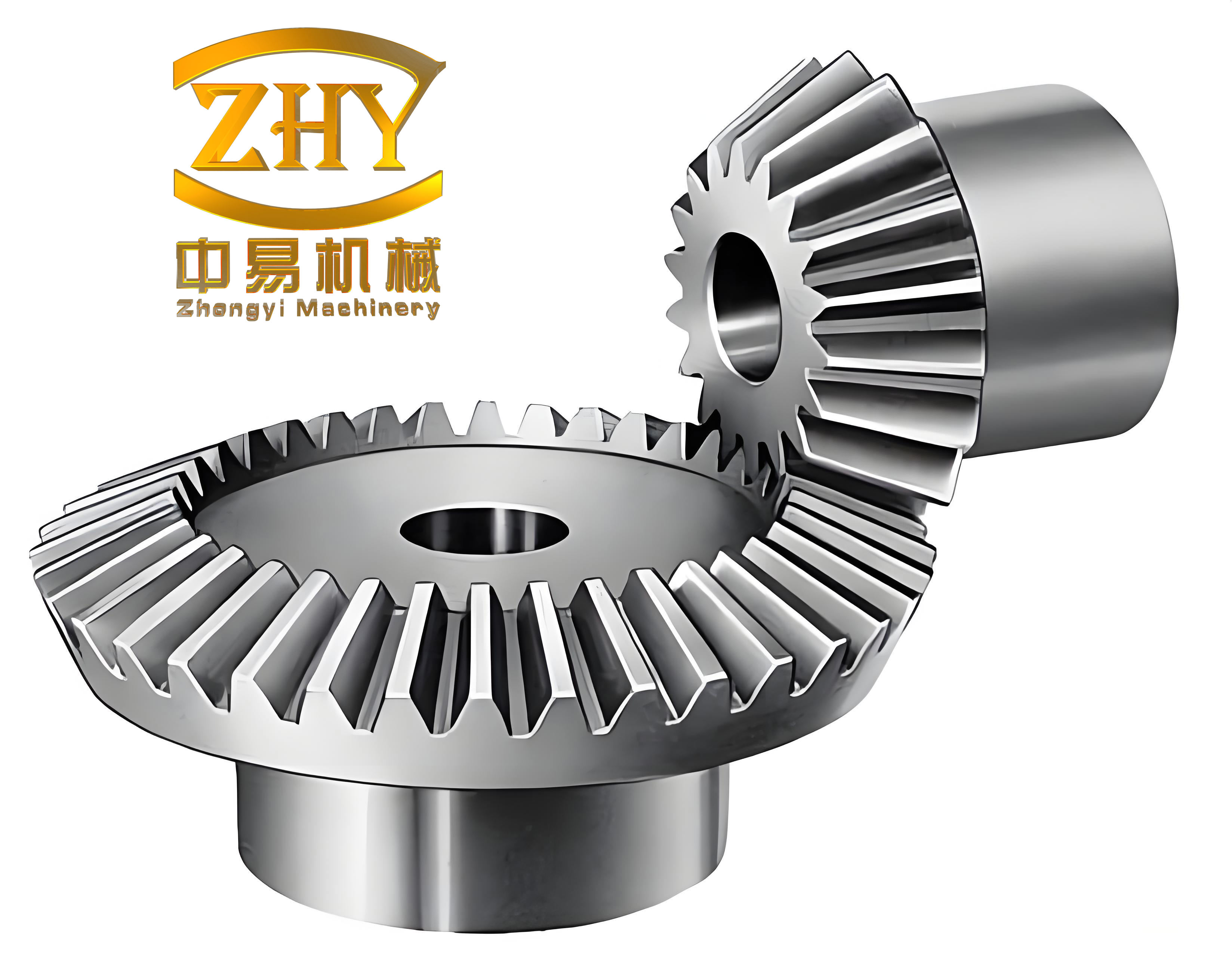
Parametric Representation and Coordinate Frames
I describe the straight bevel gear tooth surface in a fixed coordinate system Oxyz. The gear axis is aligned with the z axis. A second fixed coordinate system Otxtytzt is parallel to Oxyz and is separated from it by an axial distance u. Thus the translation from Ot to O is written as a vector along the z direction. A moving coordinate system Omxmymzm is attached to the pitch cone. Its zm axis is parallel to the gear axis, and its ym axis is tangent to the pitch cone. A second moving system Onxnynzn remains parallel to the fixed frames. The rotation between the two moving frames is parameterized by the angle φ.
The tooth surface point M is reached from a point on the pitch cone by a normal vector. I let the normal vector be l⃗. Its length is l, and its direction is defined by two angles β and λ. The angle β is measured from the ym axis, and λ describes the orientation of the normal in the plane perpendicular to ym. The unit normal vector in the moving frame is therefore
$$ \vec{n}_l = \begin{bmatrix} \sin\beta \cos\lambda \\ \cos\beta \\ -\sin\beta \sin\lambda \end{bmatrix}. $$
The full normal vector is
$$ \vec{l} = l \, \vec{n}_l = \begin{bmatrix} l\sin\beta \cos\lambda \\ l\cos\beta \\ -l\sin\beta \sin\lambda \end{bmatrix}. $$
The position vector of the tooth surface point in the fixed frame is obtained by rotating the normal vector into the intermediate moving frame, translating by the pitch radius, and translating by the axial distance. I write this as
$$ \vec{R}(\phi,u) = M_{nm}(\phi)\vec{l} + M_{tn}(u\tan\delta) + M_{st}(u). $$
The rotation matrix from Omxmymzm to Onxnynzn is
$$ M_{nm}(\phi) = \begin{bmatrix} \sin\phi & -\cos\phi & 0 \\ \cos\phi & \sin\phi & 0 \\ 0 & 0 & 1 \end{bmatrix}. $$
The translation from the moving frame to the intermediate fixed frame is
$$ M_{tn}(u\tan\delta) = \begin{bmatrix} u\tan\delta \sin\phi \\ u\tan\delta \cos\phi \\ 0 \end{bmatrix}. $$
The final translation to the fixed frame is
$$ M_{st}(u) = \begin{bmatrix} 0 \\ 0 \\ u \end{bmatrix}. $$
Here δ is the pitch cone angle of the straight bevel gear. The product u tan δ is the pitch radius at the axial section defined by u. This relation is essential because it couples the axial parameter to the radial position on the pitch cone.
Expanding the matrix expression gives the coordinate components of the tooth surface:
$$ \vec{R}(\phi,u) = \begin{bmatrix} \sin\phi \left(l\sin\beta\cos\lambda\right) – \cos\phi \left(l\cos\beta\right) + u\tan\delta\sin\phi \\ \cos\phi \left(l\sin\beta\cos\lambda\right) + \sin\phi \left(l\cos\beta\right) + u\tan\delta\cos\phi \\ -l\sin\beta\sin\lambda + u \end{bmatrix}. $$
The unit normal in the fixed frame is obtained by applying the same rotation matrix to the unit normal in the moving frame:
$$ \vec{n} = M_{nm}(\phi)\vec{n}_l = \begin{bmatrix} \sin\phi \sin\beta\cos\lambda – \cos\phi \cos\beta \\ \cos\phi \sin\beta\cos\lambda + \sin\phi \cos\beta \\ -\sin\beta \sin\lambda \end{bmatrix}. $$
This normal vector is the foundation of the method. It contains the complete local geometry of the straight bevel gear tooth surface. The position vector contains the global geometry. The relationship between them is enforced by the meshing conditions.
| Symbol | Meaning | Role in the formulation |
|---|---|---|
| φ | Rotation parameter of the moving frame | Controls the angular position around the straight bevel gear axis |
| u | Axial parameter | Controls the axial section and the pitch radius u tan δ |
| δ | Pitch cone angle | Defines the pitch cone of the straight bevel gear |
| δb | Base cone angle | Used for spherical involute tooth surfaces |
| β | Direction angle of the normal | Measured from the ym axis |
| λ | Direction angle of the normal | Orients the normal in the plane perpendicular to ym |
| l | Normal length | Distance from the pitch cone point to the tooth surface point |
| R⃗ | Position vector of the tooth surface | Defines the straight bevel gear tooth surface in Oxyz |
| n⃗ | Unit normal of the tooth surface | Defines the local orientation of the straight bevel gear tooth surface |
| r | Pitch radius | r = u tan δ |
Normal Vector Field and Meshing Conditions
The normal vector field of a straight bevel gear tooth surface is not arbitrary. It must satisfy the kinematic condition that the normal is orthogonal to the velocity of the surface point during the generating motion. I enforce this condition in two independent directions. The first condition is obtained by differentiating the position vector with respect to the rotation parameter φ. The second condition is obtained by differentiating with respect to the axial parameter u. These conditions are
$$ \vec{R}’_\phi \cdot \vec{n} = 0, $$
$$ \vec{R}’_u \cdot \vec{n} = 0. $$
After substituting the position vector and the normal vector, the first condition reduces to a differential equation for the normal length with respect to the rotation parameter:
$$ \frac{\partial l}{\partial \phi} = u \tan\delta \cos\beta. $$
The second condition reduces to a differential equation for the normal length with respect to the axial parameter:
$$ \frac{\partial l}{\partial u} = \frac{\sin\beta}{\cos\delta} \sin(\lambda – \delta). $$
These two equations are the core of the normal-vector-based generation method. They show that the geometry of the straight bevel gear tooth surface is determined by the interaction between the normal length l and the direction angles β and λ. If any one of these three quantities is prescribed as a function of φ and u, the other two can be found by integration or by algebraic solution of the two equations.
An initial condition is required for the integration. I use
$$ l(0,u) = l_0(u). $$
This initial condition defines the normal length at the starting angular position. In a practical design, l0 can be chosen to match a desired tooth thickness, a desired contact pattern, or a known reference surface. The differential equations then propagate this initial information across the entire straight bevel gear tooth surface.
| Condition | Equation | Physical meaning |
|---|---|---|
| Rotation condition | R⃗’φ · n⃗ = 0 | The normal is orthogonal to the velocity in the rotational direction |
| Axial condition | R⃗’u · n⃗ = 0 | The normal is orthogonal to the velocity in the axial direction |
| Rotation result | ∂l/∂φ = u tan δ cos β | Relates normal length growth to rotation and normal direction |
| Axial result | ∂l/∂u = (sin β / cos δ) sin(λ – δ) | Relates normal length growth to axial position and normal direction |
General Solution Procedure
The general solution procedure for a straight bevel gear tooth surface follows directly from the two differential equations. I first select the design function. The design function can be the normal length l, the direction angle β, or the direction angle λ. The choice determines which equations are algebraic and which are differential. In all cases, the final surface is obtained from the same position vector and the same normal vector.
If the normal length is prescribed, then l = f(φ,u). The partial derivatives of l are known. The rotation equation gives
$$ \cos\beta = \frac{1}{u\tan\delta} \frac{\partial l}{\partial \phi}. $$
The axial equation gives
$$ \sin(\lambda – \delta) = \frac{\cos\delta}{\sin\beta} \frac{\partial l}{\partial u}. $$
Thus β and λ are determined algebraically from the prescribed normal length. This is a powerful way to design a straight bevel gear tooth surface because the normal length directly controls the offset between the pitch cone and the tooth surface.
If the direction angle β is prescribed, then β = f(φ,u). The rotation equation becomes an ordinary differential equation for l along φ:
$$ \frac{\partial l}{\partial \phi} = u\tan\delta \cos\beta. $$
Integrating with respect to φ gives l up to an initial function of u. Once l is known, the axial equation gives λ through
$$ \sin(\lambda – \delta) = \frac{\cos\delta}{\sin\beta} \frac{\partial l}{\partial u}. $$
This approach is useful when the designer wants to control the normal direction directly, for example to shape the contact pattern of the straight bevel gear.
If the direction angle λ is prescribed, then λ = f(φ,u). The two equations become a coupled system for l and β:
$$ \frac{\partial l}{\partial \phi} = u\tan\delta \cos\beta, $$
$$ \frac{\partial l}{\partial u} = \frac{\sin\beta}{\cos\delta} \sin(\lambda – \delta). $$
This system is more delicate because compatibility conditions must be satisfied. However, it offers the most direct control over the angular orientation of the normal. In practice, I solve this system numerically with a marching scheme in φ and u, using the initial condition for l and an initial condition for β.
| Prescribed function | Known quantity | Solved quantities | Equations used |
|---|---|---|---|
| l = f(φ,u) | ∂l/∂φ, ∂l/∂u | β, λ | cos β = (∂l/∂φ)/(u tan δ); sin(λ-δ) = (cos δ/sin β) ∂l/∂u |
| β = f(φ,u) | β | l, λ | Integrate ∂l/∂φ = u tan δ cos β; then solve for λ |
| λ = f(φ,u) | λ | l, β | Coupled system ∂l/∂φ = u tan δ cos β and ∂l/∂u = (sin β/cos δ) sin(λ-δ) |
Once the three fields l, β, and λ are known as functions of φ and u, the straight bevel gear tooth surface is evaluated directly from
$$ \vec{R}(\phi,u) = \begin{bmatrix} \sin\phi \left(l\sin\beta\cos\lambda\right) – \cos\phi \left(l\cos\beta\right) + u\tan\delta\sin\phi \\ \cos\phi \left(l\sin\beta\cos\lambda\right) + \sin\phi \left(l\cos\beta\right) + u\tan\delta\cos\phi \\ -l\sin\beta\sin\lambda + u \end{bmatrix}. $$
The unit normal at each point is evaluated from
$$ \vec{n} = \begin{bmatrix} \sin\phi \sin\beta\cos\lambda – \cos\phi \cos\beta \\ \cos\phi \sin\beta\cos\lambda + \sin\phi \cos\beta \\ -\sin\beta \sin\lambda \end{bmatrix}. $$
Because the position and normal are generated from the same normal vector field, the resulting straight bevel gear tooth surface is consistent with the prescribed normal direction. This consistency is important for contact analysis, because the normal direction determines the contact kinematics.
Spherical Involute Straight Bevel Gear
The spherical involute straight bevel gear is a natural benchmark for the normal-vector method. I can recover it by choosing the normal length and the direction angles according to the spherical involute geometry. For a base cone angle δb, the spherical involute generation gives
$$ \psi = \phi \sin\delta_b, $$
$$ l = \frac{u}{\cos\delta} \sin(\phi \sin\delta_b). $$
Substituting these expressions into the differential equations gives the corresponding direction angles:
$$ \cos\beta = \frac{\sin\delta_b}{\sin\delta} \cos(\phi \sin\delta_b), $$
$$ \sin(\lambda – \delta) = \frac{\sin(\phi \sin\delta_b)}{\sin\beta}. $$
These formulas show that the spherical involute straight bevel gear is a special case of the normal-vector method. The normal length varies sinusoidally with the rotation parameter, and the direction angle β is determined by the base cone angle and the pitch cone angle. The direction angle λ follows from the axial equation. When these expressions are inserted into the position vector, the resulting surface is the classical spherical involute tooth surface of a straight bevel gear.
| Quantity | Spherical involute expression |
|---|---|
| ψ | φ sin δb |
| l | (u / cos δ) sin(φ sin δb) |
| cos β | (sin δb / sin δ) cos(φ sin δb) |
| sin(λ – δ) | sin(φ sin δb) / sin β |
I have evaluated this case for a straight bevel gear with pressure angle α0 = π/9, pitch cone angle δ = 5π/36, and number of teeth z = 18. The base cone angle is chosen according to the spherical involute relation for the given pressure angle. The resulting tooth surface is smooth, periodic in φ, and consistent with the classical spherical involute geometry. The normal-vector method reproduces the expected tooth shape without requiring a separate derivation of the involute equation. This demonstrates that the method is not limited to a special construction; it contains the classical straight bevel gear tooth surface as one of its solutions.
Polynomial Direction-Angle Families for Straight Bevel Gear Design
The real advantage of the normal-vector method appears when I use it to design non-involute straight bevel gear tooth surfaces. I can prescribe the direction angle β as a polynomial in the two parameters φ and u. A general bilinear form is
$$ \beta(\phi,u) = a_0 + a_1 u + a_2 \phi + a_3 u\phi. $$
Here a0, a1, a2, and a3 are design constants. By changing these constants, I can generate a whole family of straight bevel gear tooth surfaces. The normal length is obtained by integrating the rotation equation:
$$ \frac{\partial l}{\partial \phi} = u\tan\delta \cos\beta(\phi,u). $$
After integration, the axial equation gives the direction angle λ:
$$ \sin(\lambda – \delta) = \frac{\cos\delta}{\sin\beta} \frac{\partial l}{\partial u}. $$
This procedure is straightforward and can be implemented numerically. It allows me to design a straight bevel gear with a controlled normal direction rather than a controlled profile curve. The resulting tooth surface may be non-involute, but it still satisfies the meshing conditions and can be used for motion transmission.
| Case | a0 | a1 | a2 | a3 | β(φ,u) |
|---|---|---|---|---|---|
| Constant direction | 0.349 | 0 | 0 | 0 | 0.349 |
| Linear in rotation | 0.349 | 0 | 0.3 | 0 | 0.349 + 0.3φ |
| Linear in axial position | 0.349 | 0.01 | 0 | 0 | 0.349 + 0.01u |
| Bilinear | a0 | a1 | a2 | a3 | a0 + a1u + a2φ + a3uφ |
I have studied three representative polynomial cases for a straight bevel gear with pitch cone angle δ = 5π/36 and number of teeth z = 18. The constant direction case gives a tooth surface that is close to a simple conical surface. The linear rotation case introduces a gradual change in the normal direction as the angular parameter increases. The linear axial case introduces a gradual change in the normal direction as the axial parameter increases. The resulting tooth surfaces are different in shape, contact behavior, and manufacturability. This confirms that the normal-vector method is an active design tool: by changing a small number of coefficients, I can create different straight bevel gear tooth surfaces without changing the basic solution framework.
The polynomial family is not restricted to linear or bilinear forms. I can use higher-order polynomials, trigonometric functions, or spline functions. The only requirement is that the chosen normal direction function is smooth enough for numerical integration and that the resulting surface does not self-intersect. In practice, I recommend starting with low-order polynomials and then refining the coefficients based on contact analysis and stress analysis.
Numerical Implementation and Solid Modeling
I implement the normal-vector method as a parametric surface generator for straight bevel gear teeth. The input parameters are the pitch cone angle δ, the axial range u ∈ [umin, umax], the angular range φ ∈ [φmin, φmax], and the design function for l, β, or λ. The output is a grid of surface points and normal vectors. The grid is then used to build a solid model of a single tooth or a complete straight bevel gear.
The numerical procedure is as follows. First, I discretize the parameter domain into a rectangular grid. Second, I evaluate the prescribed design function at each grid point. Third, I integrate the differential equations along the φ direction using a Runge-Kutta scheme or a predictor-corrector scheme. Fourth, I solve the algebraic equation for the remaining direction angle. Fifth, I compute the position vector and the normal vector at each grid point. Sixth, I assemble the tooth surface patches and mirror them to form the full tooth. Seventh, I trim the tooth surface with the root cone, the face cone, and the heel and toe boundaries. Finally, I export the surface to a CAD environment for solid modeling and contact simulation.
| Step | Operation | Output |
|---|---|---|
| 1 | Discretize φ and u | Parameter grid |
| 2 | Evaluate prescribed design function | Known field on the grid |
| 3 | Integrate differential equations | l, β, or λ on the grid |
| 4 | Solve remaining direction angle | Complete normal field |
| 5 | Evaluate position and normal vectors | Surface point cloud |
| 6 | Assemble and mirror tooth surface | Single tooth surface |
| 7 | Trim with root, face, heel, and toe boundaries | Finished tooth surface |
| 8 | Export to CAD | Solid model of straight bevel gear |
The numerical accuracy depends on the step size in φ and u. Because the differential equations are first-order and relatively smooth, a moderate number of grid points is usually sufficient. I typically use a 200 by 200 grid for analysis and a finer grid for final solid modeling. The normal vector is computed analytically from the direction angles, so the surface normal does not suffer from finite-difference noise. This is a significant advantage for contact analysis, because the contact normal must be accurate.
For solid modeling, the tooth surface is generated as a parametric patch. The patch is bounded by the root cone, the face cone, and the two lateral boundaries. The lateral boundaries are obtained by evaluating the surface at the start and end of the angular parameter. The root and face boundaries are obtained by evaluating the surface at the minimum and maximum axial parameters. The resulting patch can be thickened, trimmed, and patterned around the gear axis to create a complete straight bevel gear. The method is compatible with standard CAD kernels because it produces a parametric surface with an explicit normal vector field.
Sensitivity and Design Implications
The normal-vector method provides a direct way to study how changes in the normal direction affect the straight bevel gear tooth surface. I can perform sensitivity analysis by differentiating the surface equations with respect to the design coefficients. For the polynomial family, the sensitivity of the surface to a0, a1, a2, and a3 can be computed analytically or numerically. This is useful for optimization because it tells the designer which coefficients have the strongest effect on the tooth shape.
In general, the coefficient a0 shifts the average normal direction. The coefficient a1 changes the normal direction along the axial direction, which affects the tooth thickness and the contact pattern near the heel and toe. The coefficient a2 changes the normal direction along the rotation direction, which affects the tooth curvature and the contact path. The coefficient a3 introduces a coupled effect that can be used to fine-tune the contact pattern. By combining these effects, I can design a straight bevel gear with a desired contact pattern, a desired transmission error, or a desired stress distribution.
| Design coefficient | Primary effect on the straight bevel gear tooth surface |
|---|---|
| a0 | Shifts the average normal direction and the overall tooth thickness |
| a1 | Changes the normal direction along the axial direction; affects heel-to-toe contact |
| a2 | Changes the normal direction along the rotation direction; affects curvature and contact path |
| a3 | Introduces a coupled axial-rotational effect for fine-tuning |
The sensitivity analysis also reveals limitations. If the prescribed normal direction varies too rapidly, the normal length may become negative or the surface may self-intersect. Therefore, the design coefficients must be chosen within a feasible range. I recommend checking the sign of l, the determinant of the surface metric, and the angle between the normal and the surface tangent vectors. These checks ensure that the resulting straight bevel gear tooth surface is physically meaningful.
Comparison with Conventional Approaches
Conventional methods for straight bevel gear tooth surface generation usually start from a profile curve, such as a spherical involute or a circular arc, and then sweep or rotate that curve to form the surface. The normal vector is obtained after the surface is constructed. In contrast, the normal-vector method starts from the normal vector and constructs the surface by integrating the meshing conditions. This reversal has several advantages.
First, the normal-vector method is general. It does not depend on a particular profile curve. The spherical involute is one solution, but polynomial direction-angle functions and other smooth functions are also valid. Second, the method is direct. The designer can prescribe the normal direction, which is the quantity that controls contact behavior. Third, the method is compatible with optimization. The design coefficients appear explicitly in the normal direction function, so sensitivity analysis and optimization can be performed without rebuilding the surface from scratch. Fourth, the method produces an explicit normal vector field, which is essential for accurate contact analysis and for manufacturing simulations.
| Aspect | Conventional profile-based method | Normal-vector method |
|---|---|---|
| Starting quantity | Profile curve | Normal vector field |
| Surface construction | Sweep or rotate profile | Integrate meshing conditions |
| Normal vector | Derived after surface construction | Prescribed or solved directly |
| Design flexibility | Limited to selected profile families | General smooth normal direction functions |
| Optimization | Usually requires re-parameterization | Design coefficients appear explicitly |
| Contact analysis | Normal may be less accurate if surface is discrete | Normal is analytic and consistent |
The normal-vector method is not intended to replace conventional methods in all cases. For standard spherical involute straight bevel gears, conventional methods are well established and efficient. However, for non-standard straight bevel gears, high-contact-ratio designs, and application-specific tooth surfaces, the normal-vector method offers a new degree of freedom. It allows the designer to specify the normal behavior directly and to generate the corresponding tooth surface systematically.
Conclusion
I have developed a normal-vector-based method for generating the tooth surfaces of a straight bevel gear. The method uses the normal length and the two direction angles of the tooth surface normal as the primary design variables. By enforcing the meshing conditions in the rotational and axial directions, I obtain two first-order differential equations that relate the normal length to the direction angles. These equations can be solved by prescribing any one of the three quantities: the normal length, the direction angle β, or the direction angle λ. The resulting position vector and normal vector give a complete parametric description of the straight bevel gear tooth surface.
The method reproduces the classical spherical involute straight bevel gear as a special case. It also generates non-involute straight bevel gear tooth surfaces through polynomial direction-angle functions. The polynomial family demonstrates that the method is an active design tool: by changing a few coefficients, the designer can create different tooth surfaces with different contact characteristics. The method is suitable for numerical implementation, solid modeling, and contact analysis. It provides a new way to design and analyze straight bevel gear tooth surfaces without being limited to a pre-selected profile curve.
Future work can extend the method in several directions. One direction is to couple the normal-vector method with loaded contact analysis and optimize the design coefficients for minimum transmission error and maximum load capacity. Another direction is to include manufacturing constraints, such as cutter geometry and machine tool motions, so that the designed straight bevel gear tooth surface can be produced efficiently. A third direction is to extend the method to spiral bevel gears and hypoid gears, where the normal vector field is more complex but the same general principle applies. I expect that the normal-vector method will become a useful addition to the existing toolbox for straight bevel gear design and analysis.