
In the pursuit of enhanced automotive efficiency, reducing power losses in drivetrain components is paramount. Among these, churning losses in rear axle hyperbolic gears represent a significant yet often overlooked source of energy dissipation. These losses occur as the rotating gear agitates the lubricating oil bath, converting mechanical energy into heat and fluid motion. This study, conducted from a first-person research perspective, delves into the numerical simulation of churning power losses within a passenger car rear axle housing a hyperbolic gear set. The primary objective is to elucidate the underlying flow physics, quantify the impact of key operational parameters, and propose a structural optimization to mitigate these losses. The hyperbolic gear, with its complex curved teeth enabling smooth torque transfer between non-parallel shafts, is central to this investigation. Its interaction with the oil sump is a classic multiphase flow problem, demanding sophisticated computational fluid dynamics (CFD) techniques for accurate analysis.
The numerical framework employed here is built upon the fundamental laws of fluid mechanics. The flow is treated as three-dimensional, unsteady, and incompressible. The governing equations are the continuity equation, ensuring mass conservation, and the Navier-Stokes momentum equations, describing the balance of forces. They are expressed as:
$$ \nabla \cdot \vec{V} = 0 $$
$$ \rho \frac{\partial \vec{V}}{\partial t} + \rho (\vec{V} \cdot \nabla) \vec{V} = -\nabla P + \nabla \cdot \left( \mu \left( \nabla \vec{V} + (\nabla \vec{V})^T \right) \right) + \rho \vec{g} + \vec{F} $$
Here, \(\vec{V}\) denotes the velocity vector field, \(\rho\) the fluid density, \(P\) the pressure, \(\mu\) the dynamic viscosity, \(\vec{g}\) gravitational acceleration, and \(\vec{F}\) encompasses any additional body forces. The transient nature of the gear-oil interaction necessitates a multiphase modeling approach. The Volume of Fluid (VOF) method is adopted to track the sharp interface between the lubricating oil and the surrounding air. This method solves a continuity equation for the volume fraction of one phase (typically oil, \(\alpha_{oil}\)). The evolution of the oil volume fraction is governed by:
$$ \frac{\partial}{\partial t} (\alpha_{oil} \rho_{oil}) + \nabla \cdot (\alpha_{oil} \rho_{oil} \vec{u}_{oil}) = S_{\alpha} + (m^+ – m^-) $$
The terms \(m^+\) and \(m^-\), representing mass transfer due to phase change (e.g., cavitation), are defined by empirical models. The physical properties in each computational cell are calculated as weighted averages based on the volume fractions:
$$ \rho = \alpha_{oil} \rho_{oil} + (1 – \alpha_{oil}) \rho_{air} $$
$$ \mu = \alpha_{oil} \mu_{oil} + (1 – \alpha_{oil}) \mu_{air} $$
The highly rotational flow induced by the hyperbolic gear inevitably involves turbulence. To capture its effects without prohibitive computational cost, the RNG \(k\)-\(\epsilon\) turbulence model is utilized. This model introduces two additional transport equations for the turbulent kinetic energy \(k\) and its dissipation rate \(\epsilon\):
$$ \frac{\partial (\rho k)}{\partial t} + \frac{\partial (\rho k u_i)}{\partial x_i} = \frac{\partial}{\partial x_j} \left( \alpha_k \mu_{\text{eff}} \frac{\partial k}{\partial x_j} \right) + G_k – \rho \epsilon $$
$$ \frac{\partial (\rho \epsilon)}{\partial t} + \frac{\partial (\rho \epsilon u_i)}{\partial x_i} = \frac{\partial}{\partial x_j} \left( \alpha_{\epsilon} \mu_{\text{eff}} \frac{\partial \epsilon}{\partial x_j} \right) + C_{1\epsilon} \frac{\epsilon}{k} G_k – C_{2\epsilon} \rho \frac{\epsilon^2}{k} – R_{\epsilon} $$
In these equations, \(G_k\) is the generation of turbulent kinetic energy due to mean velocity gradients, \(\mu_{\text{eff}} = \mu + \mu_t\) is the effective viscosity (\(\mu_t = C_{\mu} \rho k^2 / \epsilon\)), and \(R_{\epsilon}\) is a specific term in the RNG model that improves accuracy for rapidly strained flows, a condition prevalent near the rotating hyperbolic gear teeth.
Constructing an accurate geometric model is the first step in the simulation workflow. The focus is on the rear axle assembly containing the passive hyperbolic gear and the differential housing. Components with minimal oil immersion, such as the pinion gear and bearings, are justifiably omitted to simplify the model and reduce mesh complexity. The fluid domain is created by extracting the void space inside the axle housing and the volume occupied by the rotating parts. The hyperbolic gear itself, with its characteristic skewed and curved teeth, presents a modeling challenge. For a clearer understanding of the geometry under study, the following illustration is provided:
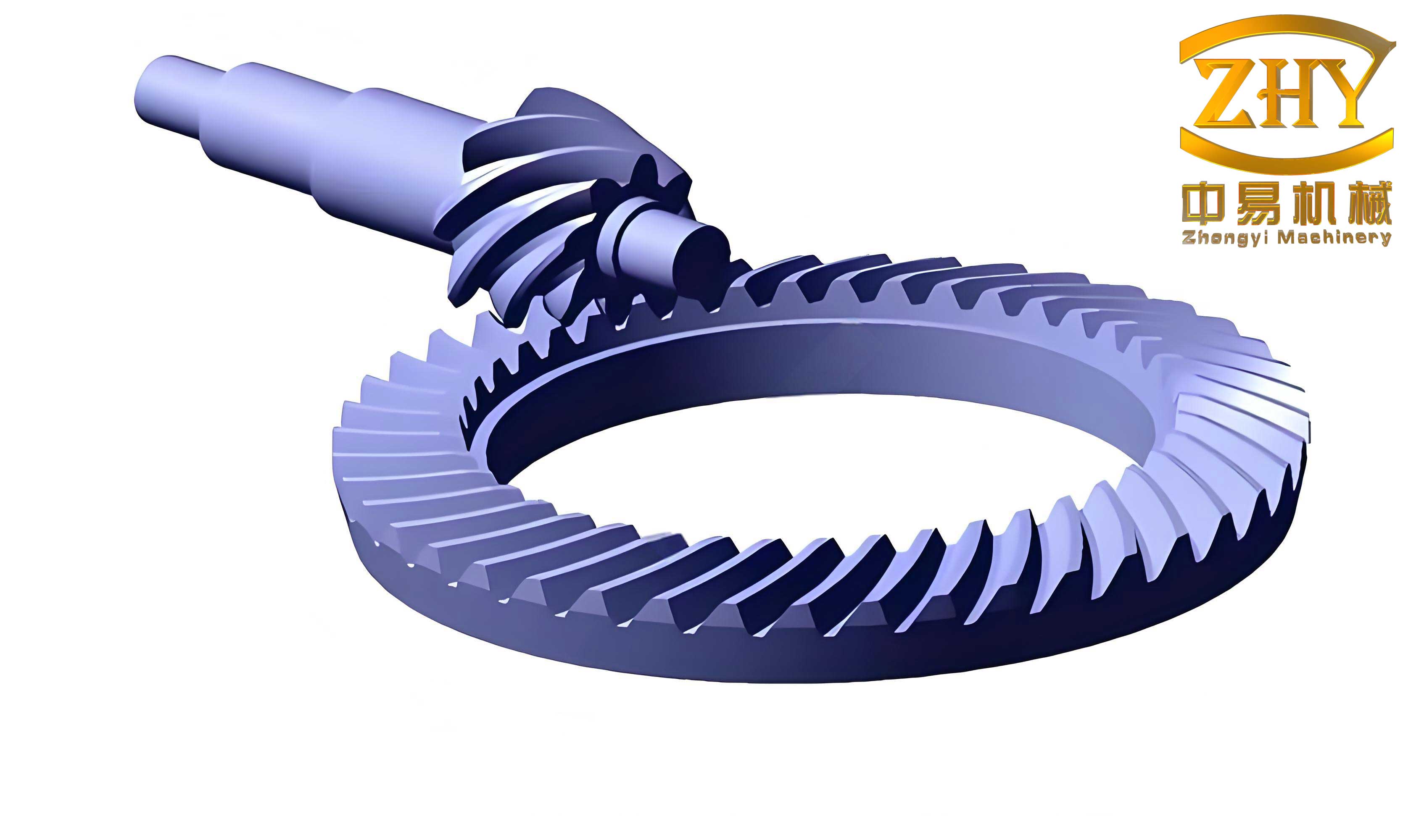
Meshing this complex domain requires a flexible strategy. An unstructured tetrahedral mesh is generated, with significant local refinement applied in the critical regions around the hyperbolic gear teeth and the differential housing. This ensures adequate resolution of the high-velocity gradients and the oil-air interface. The initial mesh contains approximately 1.37 million cells. A mesh independence study, though not detailed in the core reference, is an essential step; typically, simulations are run on progressively finer meshes until key outputs like torque converge. Boundary conditions are set to replicate the physical scenario: the outer axle and reducer housings are stationary walls with a no-slip condition; the openings at the axle ends are defined as pressure outlets at atmospheric pressure; and the passive hyperbolic gear along with the differential housing are assigned a rotational speed using a user-defined profile. The initial condition specifies a quiescent oil bath with a defined immersion depth, typically set to submerge the hyperbolic gear teeth partially.
The materials involved have distinct properties critical to the simulation’s accuracy. Lubricating oil viscosity is highly temperature-dependent, a factor central to this study. The key parameters are summarized in the table below.
| Parameter | Symbol / Unit | Value |
|---|---|---|
| Lubricating Oil Density (at 90°C) | \(\rho_{oil}\) (kg/m³) | 900 |
| Lubricating Oil Dynamic Viscosity (at 90°C) | \(\mu_{oil}\) (Pa·s) | 0.0135 |
| Air Density | \(\rho_{air}\) (kg/m³) | 1.225 |
| Air Dynamic Viscosity | \(\mu_{air}\) (Pa·s) | 1.7894 × 10⁻⁵ |
| Gravitational Acceleration | \(g\) (m/s²) | 9.81 |
| Primary Simulation Temperatures | \(T\) (°C) | 30, 60, 90 |
| Hyperbolic Gear Rotational Speeds | \(N\) (rpm) | 133, 284, 444, 621, 888, 1065 |
| Initial Oil Immersion Depth | \(h\) (mm) | 48 |
The transient simulation reveals the intricate oil flow patterns within the axle housing. As the hyperbolic gear begins to rotate, viscous forces draw oil onto the tooth surfaces. This oil is carried upward, splashed against the housing walls, and forms thin films. Over successive rotations, a dynamic equilibrium is established where oil is continuously lifted, dispersed for lubrication, and drains back to the sump. The instantaneous flow field at a low speed (e.g., 133 rpm) shows oil adhering to the gear for about a quarter rotation before beginning to detach and splash. At higher speeds, the oil is flung more violently, creating a dense mist and complex vortical structures in the air space above the oil level. The presence of protruding bolt heads on the gear flange disrupts this flow, creating localized wakes and pressure variations that contribute to additional drag.
The dynamic pressure distribution on the surfaces of the hyperbolic gear and housing is a direct indicator of the fluid resistance. Simulations show that the highest pressures are not uniformly distributed but concentrated in the tooth root fillets and on the leading faces of the teeth immersed in oil. This is where the gear “pushes” against the fluid most forcefully. A quantitative analysis across speeds demonstrates a near-quadratic relationship between gear speed and the peak dynamic pressure. For instance, increasing the speed from 133 rpm to 888 rpm can cause the maximum dynamic pressure to escalate by an order of magnitude, from around 1.5 kPa to over 23 kPa. The disruptive effect of the standard bolt heads is clearly visible in pressure contours on cross-sections, showing high-pressure stagnation regions on the bolt’s upstream side and chaotic, low-pressure wake regions downstream.
The ultimate metric of interest is the churning power loss, which is the torque required to overcome fluid drag integrated over the angular velocity (\(P_{loss} = T_{drag} \cdot \omega\)). The simulation allows for the direct calculation of this torque by integrating the pressure and shear stress distributions over the wetted surfaces of the rotating hyperbolic gear and differential housing. The influence of the two primary operational variables—speed and oil temperature—is profound and can be summarized by the following empirical correlation derived from the simulation data:
$$ P_{churn} \approx C \cdot \mu(T)^{a} \cdot \omega^{b} $$
where \(C\) is a geometry-dependent constant, \(\mu(T)\) is the temperature-dependent oil viscosity, \(\omega\) is the angular velocity, and the exponents \(a\) and \(b\) are positive, with \(b\) typically between 2 and 3, indicating a stronger dependence on speed. A detailed set of results is presented in Table 2.
| Gear Speed, \(N\) (rpm) | Angular Speed, \(\omega\) (rad/s) | Churning Power Loss, \(P_{churn}\) (W) | ||
|---|---|---|---|---|
| Oil at 30°C | Oil at 60°C | Oil at 90°C | ||
| 133 | 13.9 | 5.2 | 4.1 | 3.3 |
| 284 | 29.7 | 18.7 | 14.5 | 11.8 |
| 444 | 46.5 | 52.3 | 39.8 | 32.1 |
| 621 | 65.0 | 112.5 | 84.0 | 67.0 |
| 888 | 93.0 | 287.0 | 210.0 | 165.0 |
| 1065 | 111.5 | 475.0 | 342.0 | 265.0 |
The table unequivocally shows the dramatic increase in loss with speed. For example, at 90°C, losses increase by a factor of about 80 from the lowest to the highest speed. Conversely, increasing the temperature from 30°C to 90°C, which significantly reduces oil viscosity, cuts the churning loss roughly by half across all speeds. This underscores the dual benefit of effective cooling: preventing overheating and directly reducing viscous drag on the hyperbolic gear.
The analysis pinpointed the exposed bolt heads as a clear opportunity for drag reduction. The proposed optimization involves redesigning the connection between the hyperbolic gear and the differential housing to use countersunk bolts. In this configuration, the bolt heads are recessed into the gear’s mounting flange, presenting a flush or nearly flush surface to the surrounding oil. This simple geometric change aims to streamline the flow, minimize flow separation, and reduce the pressure drag caused by the previously protruding bolts. A comparative simulation of the optimized hyperbolic gear assembly was performed under identical operating conditions.
The effectiveness of this optimization is evident in both the flow field and the quantitative results. The disturbed wake regions behind the bolts are substantially diminished. The dynamic pressure distribution becomes smoother over the gear back face. The reduction in churning power loss is calculated for each speed, and the percentage improvement is remarkably consistent. The data is consolidated in Table 3.
| Gear Speed, \(N\) (rpm) | Churning Power Loss – Standard (W) | Churning Power Loss – Optimized (W) | Absolute Reduction (W) | Percentage Reduction |
|---|---|---|---|---|
| 133 | 3.3 | 3.1 | 0.2 | 6.1% |
| 284 | 11.8 | 10.9 | 0.9 | 7.6% |
| 444 | 32.1 | 30.9 | 1.2 | 3.7% |
| 621 | 67.0 | 61.7 | 5.3 | 7.9% |
| 888 | 165.0 | 155.0 | 10.0 | 6.1% |
| 1065 | 265.0 | 243.3 | 21.7 | 8.2% |
Note: Values are for an oil temperature of 90°C. The percentage reduction varies but consistently shows a benefit, averaging around 6-7%. This translates directly to a lower torque requirement for rotating the hyperbolic gear assembly, implying higher mechanical efficiency.
To conclusively validate the numerical predictions and the proposed optimization, a physical bench test was designed and executed. The core metric measured was the overall transmission efficiency of the rear axle assembly. Two identical axle units were prepared—one with the standard hyperbolic gear and bolt configuration, and one with the optimized countersunk bolt design. The test rig consisted of a drive motor, high-precision torque/speed sensors on the input and both output half-shafts, and a controlled loading system. The transmission efficiency \(\eta\) is calculated from the measured data using the power balance formula:
$$ \eta = \frac{P_{\text{out}}}{P_{\text{in}}} \times 100\% = \frac{\omega_{\text{out1}} \tau_{\text{out1}} + \omega_{\text{out2}} \tau_{\text{out2}}}{\omega_{\text{in}} \tau_{\text{in}}} \times 100\% $$
where \(\omega\) and \(\tau\) represent angular velocity and torque, respectively, with subscripts ‘in’ for input and ‘out1/2’ for the two outputs. Tests were conducted over a matrix of input torques (e.g., 81 Nm and 135 Nm) and across the same speed range used in the simulations. The results, summarized in Table 4, confirm a tangible improvement.
| Input Torque (Nm) | Gear Speed (rpm) | Efficiency – Standard Gear (%) | Efficiency – Optimized Gear (%) | Efficiency Gain (Percentage Points) |
|---|---|---|---|---|
| 81 | 133 | 95.1 | 96.1 | +1.0 |
| 284 | 95.3 | 96.3 | +1.0 | |
| 444 | 95.5 | 96.5 | +1.0 | |
| 621 | 95.7 | 96.7 | +1.0 | |
| 888 | 95.8 | 96.9 | +1.1 | |
| 1065 | 95.9 | 97.0 | +1.1 | |
| 135 | 133 | 95.5 | 96.5 | +1.0 |
| 284 | 95.7 | 96.7 | +1.0 | |
| 444 | 95.9 | 96.9 | +1.0 | |
| 621 | 96.1 | 97.1 | +1.0 | |
| 888 | 96.2 | 97.2 | +1.0 | |
| 1065 | 96.3 | 97.3 | +1.0 |
The data demonstrates that the optimization of the hyperbolic gear assembly yielded a consistent increase in transmission efficiency of approximately 1.0 to 1.1 percentage points across a wide operating range. This experimental finding strongly corroborates the CFD-predicted reduction in churning loss, validating the entire numerical approach and the effectiveness of the relatively simple structural change.
In summary, this comprehensive investigation successfully applied advanced CFD techniques to model the complex multiphase flow associated with churning loss in an automotive rear axle hyperbolic gear. The numerical model, incorporating the VOF method and RNG \(k\)-\(\epsilon\) turbulence model, proved capable of capturing the transient oil distribution and dynamic pressure fields. The study quantified the dominant influence of hyperbolic gear rotational speed on churning loss, showing a near-cubic relationship, and the secondary, mitigating effect of higher oil temperatures. A critical insight was the significant contribution of non-aerodynamic features like protruding bolt heads to the total drag. The proposed countermeasure—replacing standard bolts with countersunk ones in the hyperbolic gear assembly—was evaluated both numerically and experimentally. The results uniformly confirmed a meaningful reduction in churning power loss, translating to a measurable gain of about 1% in overall axle transmission efficiency. This work underscores the value of detailed fluid dynamic simulation in identifying efficiency bottlenecks in mechanical systems like hyperbolic gear drives and demonstrates that even minor design modifications, when guided by such analysis, can yield valuable improvements in energy efficiency for automotive applications.