
I have focused my research on the high-frequency induction heating behavior of a heavy-duty truck transmission helical gear. The helical gear is a critical load-bearing component in a transmission system, and its surface hardness, wear resistance, and fatigue life are strongly influenced by the heat treatment process. In heavy-duty vehicles, the helical gear operates under high torque, variable load, poor lubrication, and elevated temperature. These conditions make the helical gear susceptible to bending fatigue, tooth breakage, pitting, and surface wear. Therefore, I need a reliable heat treatment route that can produce a hard surface layer and a tough core. Induction heating is one of the most effective methods for achieving this goal because it offers high heating efficiency, low energy consumption, clean operation, and good compatibility with automation. The helical gear is especially challenging because its teeth are inclined, and a conventional circular coil does not generate a magnetic field perpendicular to the tooth surface. This causes overheating at the tooth tip, insufficient heating at the tooth root, and poor uniformity along the tooth width. I designed a quarter-tooth-width contour coil and a variable-speed spiral heating strategy to address these problems. I also established a three-dimensional finite element model for electromagnetic–thermal–motion coupling. I proposed a dynamic coordinate system method to represent the variable-speed spiral motion of the helical gear. I then performed numerical simulations and experiments to evaluate the influence of geometrical, motion, and electrical parameters on the temperature field of the helical gear.
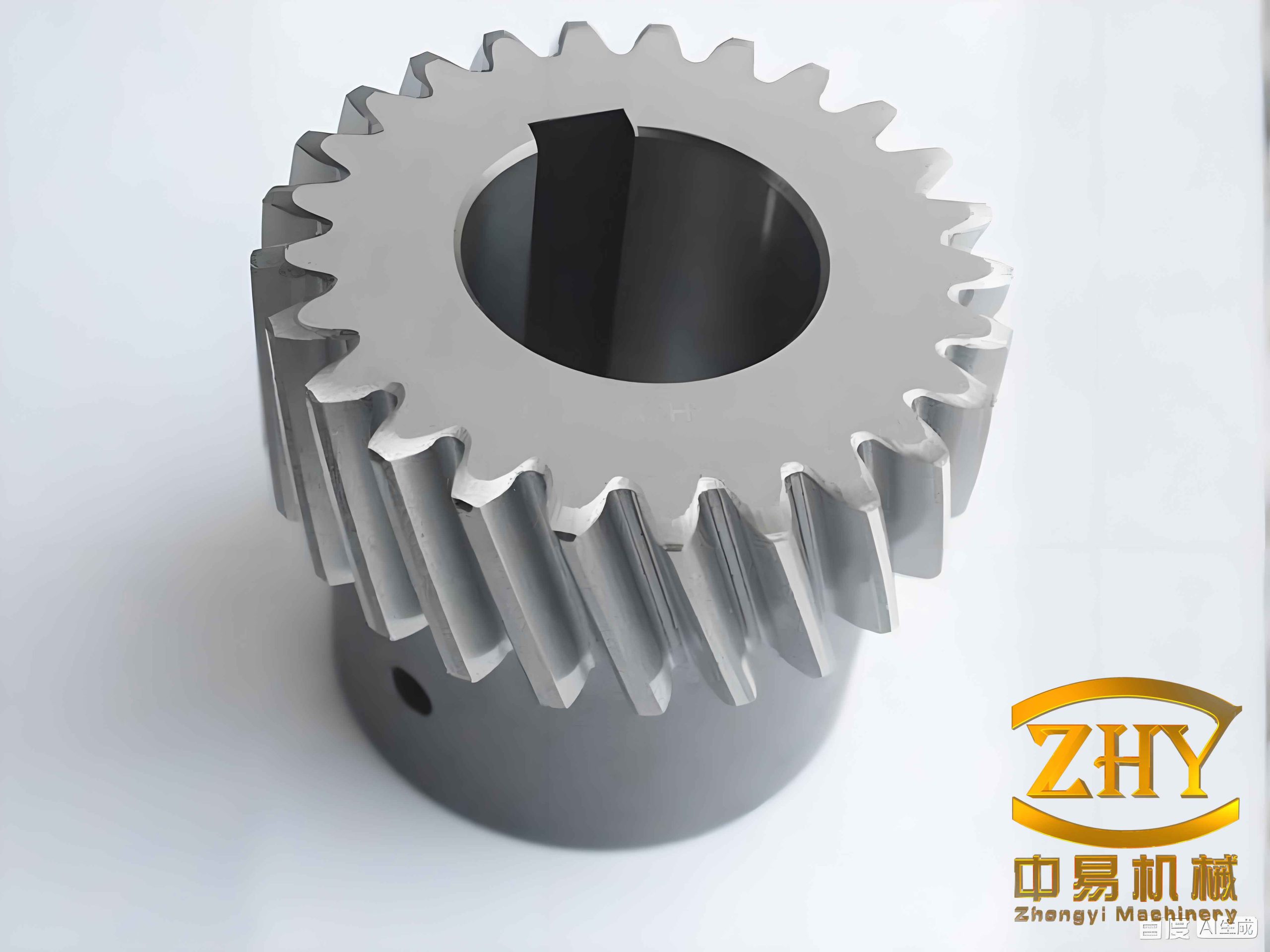
The helical gear used in this study is made of 45 steel. Its chemical composition is summarized in Table 1. The material properties are highly nonlinear with respect to temperature. I therefore used temperature-dependent data for thermal conductivity, specific heat capacity, electrical resistivity, and relative magnetic permeability. These properties determine the electromagnetic field, the induced eddy current, the Joule heat generation, and the subsequent heat conduction inside the helical gear.
| Element | C | Si | Mn | Cr | Ni | Cu |
|---|---|---|---|---|---|---|
| Mass fraction (%) | 0.42–0.50 | 0.17–0.37 | 0.50–0.80 | 0.12–0.25 | 0.18–0.30 | 0.14–0.25 |
For the numerical simulation, I treated the material properties as functions of temperature. The thermal conductivity, specific heat capacity, electrical resistivity, and relative magnetic permeability were imported into the finite element code through interpolation tables. The density was assumed to remain constant during the heating process. The initial temperature of the helical gear was set to 25 °C. The quenching temperature range was set to 850–950 °C. The Curie temperature of 45 steel is approximately 727 °C, above which the relative magnetic permeability drops sharply to approximately 1. This change reduces the induced eddy current and the Joule heat generation rate. I accounted for this effect in the coupled electromagnetic–thermal analysis.
The electromagnetic field in the induction heating process is governed by Maxwell’s equations. I used the following differential form:
$$\nabla \times \mathbf{H} = \mathbf{J} + \frac{\partial \mathbf{D}}{\partial t}$$
$$\nabla \times \mathbf{E} = -\frac{\partial \mathbf{B}}{\partial t}$$
$$\nabla \cdot \mathbf{D} = 0$$
$$\nabla \cdot \mathbf{B} = 0$$
Here, \(\mathbf{H}\) is the magnetic field intensity, \(\mathbf{J}\) is the current density, \(\mathbf{D}\) is the electric displacement, \(\mathbf{E}\) is the electric field intensity, and \(\mathbf{B}\) is the magnetic flux density. The constitutive relations are:
$$\mathbf{D} = \varepsilon \mathbf{E}$$
$$\mathbf{J} = \sigma \mathbf{E}$$
$$\mathbf{B} = \mu \mathbf{H}$$
where \(\varepsilon\) is the permittivity, \(\sigma\) is the electrical conductivity, and \(\mu\) is the magnetic permeability. I introduced the magnetic vector potential \(\mathbf{A}\) and the electric scalar potential \(\varphi\) to simplify the formulation:
$$\mathbf{B} = \nabla \times \mathbf{A}$$
$$\mathbf{E} = -\frac{\partial \mathbf{A}}{\partial t} – \nabla \varphi$$
The current density can then be expressed as:
$$\mathbf{J} = \sigma \mathbf{E} = -\sigma \frac{\partial \mathbf{A}}{\partial t} – \sigma \nabla \varphi$$
The coupled electromagnetic field equations used in my finite element model are:
$$\nabla \times \left( \frac{1}{\mu} \nabla \times \mathbf{A} \right) + \sigma \frac{\partial \mathbf{A}}{\partial t} + \sigma \nabla \varphi = 0$$
$$\nabla \cdot \left( -\sigma \frac{\partial \mathbf{A}}{\partial t} – \sigma \nabla \varphi \right) = 0$$
The eddy current penetration depth is an important parameter for the helical gear induction heating process. I used the following expression:
$$\delta = \sqrt{\frac{\rho}{\pi f \mu}}$$
where \(\delta\) is the penetration depth, \(\rho\) is the electrical resistivity, \(f\) is the current frequency, and \(\mu\) is the magnetic permeability. For a given material, the penetration depth decreases as the frequency increases. In my simulation, the frequency was set to 100 kHz for the baseline case, and I also studied 80 kHz and 120 kHz. The current density was set to \(7.5 \times 10^7\) A/m² for the baseline case, and I also studied \(6.0 \times 10^7\) A/m² and \(9.0 \times 10^7\) A/m². The induced Joule heat per unit volume is:
$$q_v = \rho J^2$$
where \(q_v\) is the internal heat source intensity. The transient heat conduction equation for the helical gear is:
$$\rho c \frac{\partial T}{\partial t} = \frac{\partial}{\partial x}\left( k \frac{\partial T}{\partial x} \right) + \frac{\partial}{\partial y}\left( k \frac{\partial T}{\partial y} \right) + \frac{\partial}{\partial z}\left( k \frac{\partial T}{\partial z} \right) + q_v$$
where \(T\) is temperature, \(c\) is specific heat capacity, \(k\) is thermal conductivity, and \(t\) is time. The boundary conditions include prescribed temperature, prescribed heat flux, convection, and radiation:
$$T = f(x,y,z,t) \quad \text{on } S_1$$
$$-k \frac{\partial T}{\partial n} = q_n \quad \text{on } S_2$$
$$-k \frac{\partial T}{\partial n} = h(T_w – T_f) \quad \text{on } S_3$$
$$-k \frac{\partial T}{\partial n} = \varepsilon \sigma (T^4 – T_0^4) \quad \text{on } S_4$$
where \(h\) is the convection heat transfer coefficient, \(T_w\) is the surface temperature, \(T_f\) is the ambient temperature, \(\varepsilon\) is the emissivity, and \(\sigma\) is the Stefan–Boltzmann constant. In my simulation, the heat exchange between the helical gear and the surrounding air included both convection and radiation. The induction coil and the air domain were not included in the thermal solution except as boundary influences, because the coil was water-cooled and its temperature was assumed to remain nearly constant.
The design of the induction coil is critical for the helical gear. The coil must ensure that the magnetic field is distributed as uniformly as possible along the tooth profile and tooth width. I followed several design principles. The coil should be made of a hollow rectangular copper tube to allow internal water cooling. The tube wall thickness should be greater than the hot penetration depth. The axial width of the copper tube determines the effective heating area. The gap between the coil and the helical gear should be as small as possible without causing contact or short circuit. The coil geometry should compensate for the helical angle of the helical gear. I evaluated four coil configurations: a circular coil, a full contour coil, a convex contour coil, and a quarter-tooth-width contour coil. The quarter-tooth-width contour coil was selected because it reduces manufacturing cost, simplifies water cooling, avoids the end effect along the tooth width, and enables layer-by-layer heating of the helical gear.
| Coil type | Advantages | Disadvantages | Decision |
|---|---|---|---|
| Circular coil | Simple structure, easy fabrication | Non-perpendicular magnetic field, tip overheating, root underheating | Rejected |
| Full contour coil | Better tooth profile conformity | High manufacturing difficulty, middle overheating along tooth width | Rejected |
| Convex contour coil | Improved tooth width uniformity | Higher power demand, lower efficiency | Rejected |
| Quarter-tooth-width contour coil | Low cost, good water cooling, reduced end effect, suitable for layer-by-layer heating | Requires precise motion control | Selected |
The quarter-tooth-width contour coil was modeled in a CAD environment and manufactured by 3D printing. The coil consists of an induction ring, a busbar, a connecting plate, and a water supply pipe. The induction ring is the effective heating part. The busbar was made curved to increase the contact area with the connecting plate and to avoid drilling holes on both sides. An insulating plate was installed between the two sides of the busbar to prevent short circuit. The coil was connected to the high-frequency power supply through the connecting plate. The cooling water flowed through the hollow copper tube to remove the heat generated by the coil itself.
| Parameter | Value |
|---|---|
| Copper tube cross-section | 10 mm × 6 mm × 2 mm |
| Coil inner distance to tooth tip | 6 mm |
| Coil inner distance to tooth root | 3 mm |
| Coil axial width | 10 mm |
| Cooling method | Internal water circulation |
| Manufacturing method | 3D printing of copper alloy |
The helical gear used in the simulation and experiment had a module of 4.5 mm, 12 teeth, a tooth width of 40 mm, and a helix angle of 10°. The pitch circle diameter was 64.4 mm. The coil was placed with a constant gap to the tooth tip and tooth root. The helical gear moved relative to the coil in a variable-speed spiral path. This motion combined axial translation and radial rotation. The instantaneous linear velocity \(v_t\) and instantaneous angular velocity \(\omega_t\) must satisfy the following relationship:
$$v_t = \omega_t r \tan \beta$$
where \(r\) is the pitch circle radius and \(\beta\) is the helix angle. This relationship ensures that the helical gear tooth surface remains parallel to the coil during the heating process. I controlled the linear and angular velocities independently through a programmable logic controller. The motion was designed as a “slow–fast–slow” profile along the tooth width. The heating layers \(d_1\), \(d_2\), \(d_3\), and \(d_4\) each had a width of 10 mm. The baseline velocities and heating times are given in Table 4.
| Heating layer | Linear velocity (m/s) | Angular velocity (rad/s) | Heating time (s) |
|---|---|---|---|
| \(d_1\) | \(1.0 \times 10^{-3}\) | \(2.0 \times 10^{-2}\) | 10 |
| \(d_2\) | \(2.5 \times 10^{-3}\) | \(5.1 \times 10^{-2}\) | 4 |
| \(d_3\) | \(2.5 \times 10^{-3}\) | \(5.1 \times 10^{-2}\) | 4 |
| \(d_4\) | \(1.0 \times 10^{-3}\) | \(2.0 \times 10^{-2}\) | 10 |
To represent the continuous variable-speed spiral motion of the helical gear in the finite element model, I proposed a dynamic coordinate system method. In this method, the helical gear is not physically translated and rotated in a single continuous step. Instead, the relative position between the coil and the helical gear is updated at discrete heating positions. At each heating position, a local coordinate system group is created for the coil. The coil is divided into a number of segments according to its contour. For each segment, I defined a local Cartesian coordinate system or a local cylindrical coordinate system. The current density load was applied along the local coordinate directions so that the current formed a closed loop around the helical gear. When the coil moved to the next heating position, the local coordinate system group was rotated by an angle \(TH\). The rotation angle was calculated as:
$$TH = \frac{s \tan \beta}{r} \times \frac{180}{\pi}$$
where \(s\) is the distance between adjacent heating positions. This method avoids the need to rebuild the entire geometry and mesh at every time step. It also allows the electromagnetic and thermal fields to be solved sequentially with good numerical stability. I used the following procedure. First, I collected the characteristic parameters of the helical gear, including the pitch radius, helix angle, tooth number, total movement distance, and distance between adjacent heating positions. Second, I divided one tooth of the coil into eight parts and established local coordinate systems at the tooth tip, both tooth flanks, the tooth root, and the root arc center. Third, I rotated these local coordinate systems by \(360/z\) degrees repeatedly to obtain the initial local coordinate system group. Fourth, I imported the discrete CAD models of the helical gear and coil into the finite element software. Fifth, I solved the electromagnetic and thermal fields at the initial heating position. Sixth, I incremented the heating position index \(i\) by one and rotated the local coordinate system group by \(TH\). Seventh, I repeated the electromagnetic and thermal solutions until all heating positions were completed. This procedure is summarized in Table 5.
| Step | Operation | Purpose |
|---|---|---|
| 1 | Collect geometric and motion parameters | Define the helical gear and coil configuration |
| 2 | Divide one coil tooth into segments | Create local coordinate systems for current loading |
| 3 | Rotate the local coordinate systems by \(360/z\) | Form the initial local coordinate system group |
| 4 | Import discrete CAD models | Represent different relative positions |
| 5 | Solve electromagnetic and thermal fields | Compute eddy current and temperature |
| 6 | Move to the next heating position | Update the relative position |
| 7 | Rotate local coordinate systems by \(TH\) | Maintain the correct current direction |
| 8 | Repeat until all positions are solved | Complete the variable-speed spiral heating |
I used the finite element method to solve the coupled electromagnetic–thermal–motion problem. For the electromagnetic analysis, I selected a 3-D edge element formulation. The helical gear, coil, and air were meshed with 20-node hexahedral solid elements. The helical gear was assigned degrees of freedom for electric potential and magnetic vector potential. The coil and air were assigned only the magnetic vector potential degree of freedom. For the thermal analysis, the helical gear was meshed with 20-node hexahedral thermal elements. The coil and air were set as null elements in the thermal analysis because their temperature changes were neglected. The mesh was refined near the tooth surface and along the tooth width. The element size in the tooth surface region was smaller than the eddy current penetration depth. The mesh became coarser toward the core of the helical gear to reduce the total number of elements. The air domain was five times larger than the helical gear volume to allow the magnetic flux lines to close properly. The outer boundary of the air domain was set to a zero magnetic vector potential condition.
| Region | Electromagnetic element | Thermal element | Material properties |
|---|---|---|---|
| Helical gear | SOLID117 | SOLID90 | Temperature-dependent \(\mu_r\), \(\rho\), \(k\), \(c\) |
| Coil | SOLID117 | NULL | Constant \(\mu_r\), \(\rho\) |
| Air | SOLID117 | NULL | Constant \(\mu_r\) |
I solved the electromagnetic field as a harmonic analysis at a fixed frequency. The induced Joule heat was then transferred to the thermal analysis as an internal heat source. The thermal analysis was transient. The time step was chosen to be small enough to capture the temperature evolution near the Curie point. The temperature field obtained from one heating position was saved and then imported as the initial condition for the next heating position. This sequential coupling procedure is expressed as:
$$T_{i+1}^{0} = T_i^{end}$$
$$q_{v,i+1} = \rho(T_{i+1}) \left| \mathbf{J}_{i+1} \right|^2$$
where \(T_{i+1}^{0}\) is the initial temperature at the next heating position, \(T_i^{end}\) is the final temperature at the previous heating position, and \(q_{v,i+1}\) is the Joule heat source at the next heating position. This approach ensures continuity of the thermal field during the variable-speed spiral motion. The electromagnetic and thermal material properties were updated at each time step according to the current temperature. The relative magnetic permeability decreased sharply above the Curie temperature, which automatically reduced the heat generation rate. I also included convection and radiation boundary conditions on the tooth surface.
I first analyzed the electromagnetic field at the initial heating position. The magnetic flux density was highest near the tooth tip and the tooth root. The tooth tip experienced the sharp corner effect, while the tooth root experienced the proximity effect because it was closer to the coil. The magnetic flux density decreased exponentially from the tooth surface toward the core. This is consistent with the skin effect. The magnetic flux density along the tooth profile was not uniform. It was highest at the tooth tip, lower at the tooth flank, and moderately high at the tooth root. The helical angle caused a slight asymmetry between the left and right tooth flanks. The left flank had a slightly higher magnetic flux density and a larger gradient than the right flank. This asymmetry is important for the helical gear because it can lead to uneven hardening along the tooth profile if the coil and motion parameters are not optimized.
I then analyzed the transient temperature field at the initial heating position. The temperature at the tooth tip increased fastest in the first 2.5 s because of the sharp corner effect. However, once the temperature exceeded the Curie point, the relative magnetic permeability dropped, and the heating rate decreased. The tooth root then became the fastest-heating region because it was closest to the coil and the proximity effect was strong. At about 4 s, both the tooth tip and the tooth root reached the austenitizing temperature. The heat generated at these regions decreased, and heat conduction transferred energy toward the tooth flank and the core. The tooth flank temperature then increased rapidly and reached the austenitizing temperature at about 6 s. After that, the temperature distribution became more uniform. At 10 s, the temperature along the tooth profile was within the quenching range of 850–950 °C. The maximum temperature difference along the tooth profile was less than 50 °C. This indicates that the quarter-tooth-width contour coil and the selected process parameters can produce a relatively uniform temperature field along the tooth profile.
The temperature distribution along the tooth width is equally important. I divided the helical gear into four heating layers along the tooth width. Each layer contained ten heating positions. The coil moved in a variable-speed spiral path. I compared the overall heating method and the layer-by-layer heating method. In the overall heating method, a full contour coil was used. The magnetic flux density was concentrated near the middle of the coil. Therefore, the middle of the tooth width became hotter than the two end faces. The maximum temperature difference along the tooth width was about 87 °C. In the layer-by-layer heating method, the quarter-tooth-width contour coil was used. The maximum temperature difference along the tooth width was about 18 °C when the starting and ending positions were properly adjusted. The layer-by-layer method also required lower power and provided better uniformity. Therefore, I selected the layer-by-layer heating method for the helical gear.
| Heating method | Coil type | Maximum temperature difference along tooth width | Heating quality |
|---|---|---|---|
| Overall heating | Full contour coil | About 87 °C | Poor uniformity |
| Layer-by-layer heating | Quarter-tooth-width contour coil | About 18 °C | Good uniformity |
I investigated the influence of the starting and ending heating positions on the temperature uniformity along the tooth width. I defined three initial positions, \(W_1\), \(W_2\), and \(W_3\). At these positions, the distance between the lower end face of the coil and the lower end face of the helical gear was 0 mm, 5 mm, and 10 mm, respectively. The results are summarized in Table 7. When the distance increased from 0 mm to 10 mm, the maximum temperature difference along the tooth width decreased from about 45 °C to about 18 °C. The reason is that a larger starting distance provides a preheating effect and increases the heating time near the end face. However, increasing the distance further also increases the total heating time and reduces production efficiency. Therefore, a distance of about 10 mm was selected as the preferred starting and ending position.
| Starting distance (mm) | Maximum temperature difference along tooth width (°C) | Observation |
|---|---|---|
| 0 | 45 | End faces too cold |
| 5 | 30 | Moderate uniformity |
| 10 | 18 | Good uniformity |
I also studied the influence of the coil moving speed on the temperature field. I compared a sudden speed change and a gradual speed change. In the sudden change mode, the coil speed changed abruptly from 1 mm/s to 2.5 mm/s. In the gradual change mode, the coil speed increased from 1 mm/s to 2.5 mm/s in steps of 0.15 mm/s per heating position. The gradual change mode produced a smoother temperature distribution and a smaller maximum temperature difference. The sudden change mode produced a temperature jump along the tooth width. I therefore selected the gradual change mode. I also varied the coil moving speed from 1 mm/s to 1.5 mm/s, 2.5 mm/s, and 3.5 mm/s. The maximum temperature difference along the tooth width decreased as the speed increased, but the decrease rate slowed down. When the speed was too high, the middle of the tooth width did not reach the quenching temperature. Therefore, an appropriate moving speed is necessary to balance uniformity and hardness depth.
| Moving speed (mm/s) | Maximum temperature difference along tooth width (°C) | Heating quality |
|---|---|---|
| 1.0 | 55 | High temperature, large difference |
| 1.5 | 40 | Improved uniformity |
| 2.5 | 28 | Good uniformity |
| 3.5 | 22 | Good uniformity but risk of underheating |
I analyzed the influence of current density on the temperature distribution along the tooth profile. The current density values were \(6.0 \times 10^7\) A/m², \(7.5 \times 10^7\) A/m², and \(9.0 \times 10^7\) A/m². The temperature at the tooth tip was the highest, followed by the tooth root, and the tooth flank was the lowest. This is due to the combined effects of the sharp corner effect and the proximity effect. As the current density increased, the maximum temperature difference along the tooth profile increased. At \(7.5 \times 10^7\) A/m², the temperature difference was moderate, and the temperature distribution was relatively uniform. At \(9.0 \times 10^7\) A/m², the temperature difference increased sharply. Therefore, I selected \(7.5 \times 10^7\) A/m² as the preferred current density.
| Current density (A/m²) | Maximum temperature difference along tooth profile (°C) | Temperature uniformity |
|---|---|---|
| \(6.0 \times 10^7\) | 35 | Moderate |
| \(7.5 \times 10^7\) | 28 | Best |
| \(9.0 \times 10^7\) | 52 | Poor |
I also studied the influence of current frequency. The frequencies were 80 kHz, 100 kHz, and 120 kHz. As the frequency increased, the skin effect became stronger, and the magnetic field was more concentrated near the surface. The temperature difference along the tooth profile increased with increasing frequency. At 80 kHz, the penetration depth was larger, and the temperature distribution was more uniform. At 120 kHz, the temperature difference was larger, especially at the tooth tip. However, the frequency also affects the hardness depth. A lower frequency generally produces a deeper hardened layer, while a higher frequency produces a shallower but harder layer. For the helical gear in this study, I found that 100 kHz provided a good compromise between hardness depth and temperature uniformity. The maximum temperature difference at 100 kHz was smaller than that at 120 kHz and larger than that at 80 kHz, but the hardness depth was more suitable for the heavy-duty application.
| Frequency (kHz) | Maximum temperature difference along tooth profile (°C) | Hardness depth tendency |
|---|---|---|
| 80 | 24 | Deeper |
| 100 | 31 | Balanced |
| 120 | 45 | Shallower |
I conducted a series of induction heating experiments to validate the numerical model. I used a high-frequency power supply with a maximum output of 35 kW and a frequency range of 40–100 kHz. The coil was the quarter-tooth-width contour coil described above. The helical gear was mounted on a three-jaw chuck. The chuck was driven by a stepper motor and a lead screw slide rail. The linear motion and rotational motion were controlled by a programmable logic controller. The cooling water was supplied to the coil and the spray ring. The temperature was measured by K-type thermocouples welded at four points on the helical gear. Point A was at the center of the tooth tip. Point B was at the intersection of the pitch circle and the right tooth flank. Point C was at the center of the tooth root. Point D was at the middle of the tooth width on the same right tooth flank as point B. The thermocouples were connected to a temperature recorder and a computer with a real-time temperature acquisition system. I ensured that the electromagnetic field did not significantly disturb the temperature measurement by performing a power interruption test. The measured temperature change was small when the power was switched off and on again, so the measurement data were considered reliable.
I compared the experimental and simulated temperature histories at points A, B, C, and D. The results are shown in Table 10. The experimental curves and simulated curves had the same overall trend. The temperature increased rapidly before the Curie point and then increased slowly after the Curie point. The tooth tip reached the highest temperature, followed by the tooth root, and the tooth flank reached the lowest temperature. The maximum temperature error was about 3.1%. The experimental temperature was slightly higher than the simulated temperature. This difference is attributed to the simplified boundary conditions in the simulation and to the eddy current loss in the thermocouples. The thermocouples themselves can be heated by the magnetic field, which increases the measured temperature. The temperature difference between the experiment and simulation was 21.3 °C at point A, 16.7 °C at point B, 20.8 °C at point C, and 20.5 °C at point D. These differences are acceptable for engineering analysis. The agreement between the experimental and simulated results confirms that the dynamic coordinate system method and the coupled electromagnetic–thermal–motion model are reliable for predicting the temperature field of the helical gear during high-frequency induction heating.
| Measurement point | Experimental temperature (°C) | Simulated temperature (°C) | Difference (°C) | Relative error |
|---|---|---|---|---|
| A (tooth tip) | 1015.3 | 994.0 | 21.3 | 2.1% |
| B (tooth flank, 2 mm depth) | 932.7 | 916.0 | 16.7 | 1.8% |
| C (tooth root) | 967.8 | 947.0 | 20.8 | 2.2% |
| D (tooth width middle) | 945.5 | 925.0 | 20.5 | 2.2% |
The experimental results also showed that the temperature at point D was slightly higher than that at point B during the early stage of heating. This is due to the helix angle of the helical gear. When the layer-by-layer heating method is used, the heating time near the end faces is shorter than that near the middle of the tooth width. This causes the end faces to receive less heat. However, by adjusting the starting and ending positions and the moving speed, I was able to reduce this difference. After the temperature reached the Curie point, the temperature difference between points B and D decreased because heat conduction transferred energy from the middle of the tooth width toward the end faces. The final temperature difference between points B and D was less than 25 °C, which is acceptable for the quenching process.
The experimental validation confirms that the numerical model can predict the temperature field of the helical gear with good accuracy. The maximum relative error was 3.1%, which is within the acceptable range for engineering applications. The model can therefore be used to optimize the induction heating process of the helical gear. The key findings of my study are summarized as follows. First, the quarter-tooth-width contour coil is more suitable for the helical gear than the full contour coil because it reduces the end effect and improves the temperature uniformity along the tooth width. Second, the layer-by-layer heating method with a variable-speed spiral motion produces a more uniform temperature field than the overall heating method. Third, the starting and ending positions should be set at a distance of about 10 mm from the end faces to provide a preheating effect and reduce the end-face temperature drop. Fourth, the coil moving speed should be gradually changed rather than suddenly changed to avoid temperature jumps. Fifth, the current density should be selected to balance heating efficiency and temperature uniformity. Sixth, the current frequency should be selected to balance hardness depth and temperature uniformity. Seventh, the dynamic coordinate system method is an effective way to simulate the variable-speed spiral motion of the helical gear in a finite element model.
I believe that this study provides a useful reference for the induction heating of heavy-duty truck transmission helical gears. The helical gear is a complex component, and its induction heating process involves multiple physical fields. The dynamic coordinate system method and the coupled electromagnetic–thermal–motion model developed in this study can be extended to other types of gears and other induction heating processes. In future work, I plan to include phase transformation and stress analysis in the model to predict the hardness profile and residual stress distribution more accurately. I also plan to use an orthogonal experimental design to optimize the process parameters more systematically. These improvements will further enhance the industrial applicability of the proposed method for the helical gear induction heating process.