
I carried out this study to understand how carburizing and quenching affect the performance of complex helical gears used in electric vehicle drivetrains. The helical gears in this work were made from 20CrMnTiH steel. My goal was to predict carbon concentration, microstructure, hardness, residual stress, and distortion during the carburizing and quenching process, and then to optimize the process parameters so that the final helical gears would meet hardness and case-depth requirements while keeping distortion and helix total deviation as low as possible. I combined a multi-field finite element model with experimental validation and then used both orthogonal experiments and a BP neural network to optimize the heat-treatment schedule. In the following sections, I present the governing equations, material parameters, meshing strategy, boundary conditions, validation results, parametric studies, and optimization outcomes in detail.
1. Background and Motivation
Carburizing and quenching is one of the most common heat-treatment routes for improving the service performance of helical gears. During carburizing, carbon atoms diffuse into the surface of the helical gears, and during subsequent quenching, the carbon-enriched surface transforms into a hard martensitic case while the core remains relatively tough. For helical gears in electric vehicles, the transmission system is expected to operate at high speed and high torque, so the requirements for surface hardness, case depth, core hardness, and dimensional accuracy are strict. Distortion is especially critical because helical gears rely on precise tooth geometry for smooth meshing and low noise. A small change in helix deviation can alter contact patterns, increase vibration, and reduce fatigue life.
The difficulty is that carburizing and quenching involve strong coupling among temperature, carbon diffusion, phase transformation, and stress/strain. The surface and the core of the helical gears do not cool at the same rate, and the carbon concentration varies with depth. As a result, martensitic transformation starts at different times in different regions. The resulting thermal stress and transformation stress can cause complex distortion. Because experimental measurement of every transient field is difficult, I used numerical simulation to predict the process and to guide optimization. The simulation tool I used was COSMAP, which is based on metallo-thermo-mechanical theory and can solve coupled temperature, diffusion, phase, and stress fields.
I also used JMatPro to obtain thermo-physical and mechanical properties of 20CrMnTiH steel, including density, specific heat, thermal conductivity, Young’s modulus, Poisson’s ratio, yield strength, hardening parameters, thermal expansion coefficients, transformation plasticity coefficients, and latent heat. The geometry of the helical gears was built with SolidWorks and KISSsoft, and the finite element mesh was generated with GiD. The heat-treatment process was designed according to industrial requirements for electric vehicle helical gears. I then validated the model against measured carbon concentration, microstructure, hardness, and helix total deviation. After validation, I studied how carburizing temperature, strong carburizing time, diffusion time, and cooling rate affect the performance of helical gears. Finally, I used orthogonal experiments and a BP neural network to identify optimal process parameters.
2. Gear Geometry, Material, and Technical Requirements
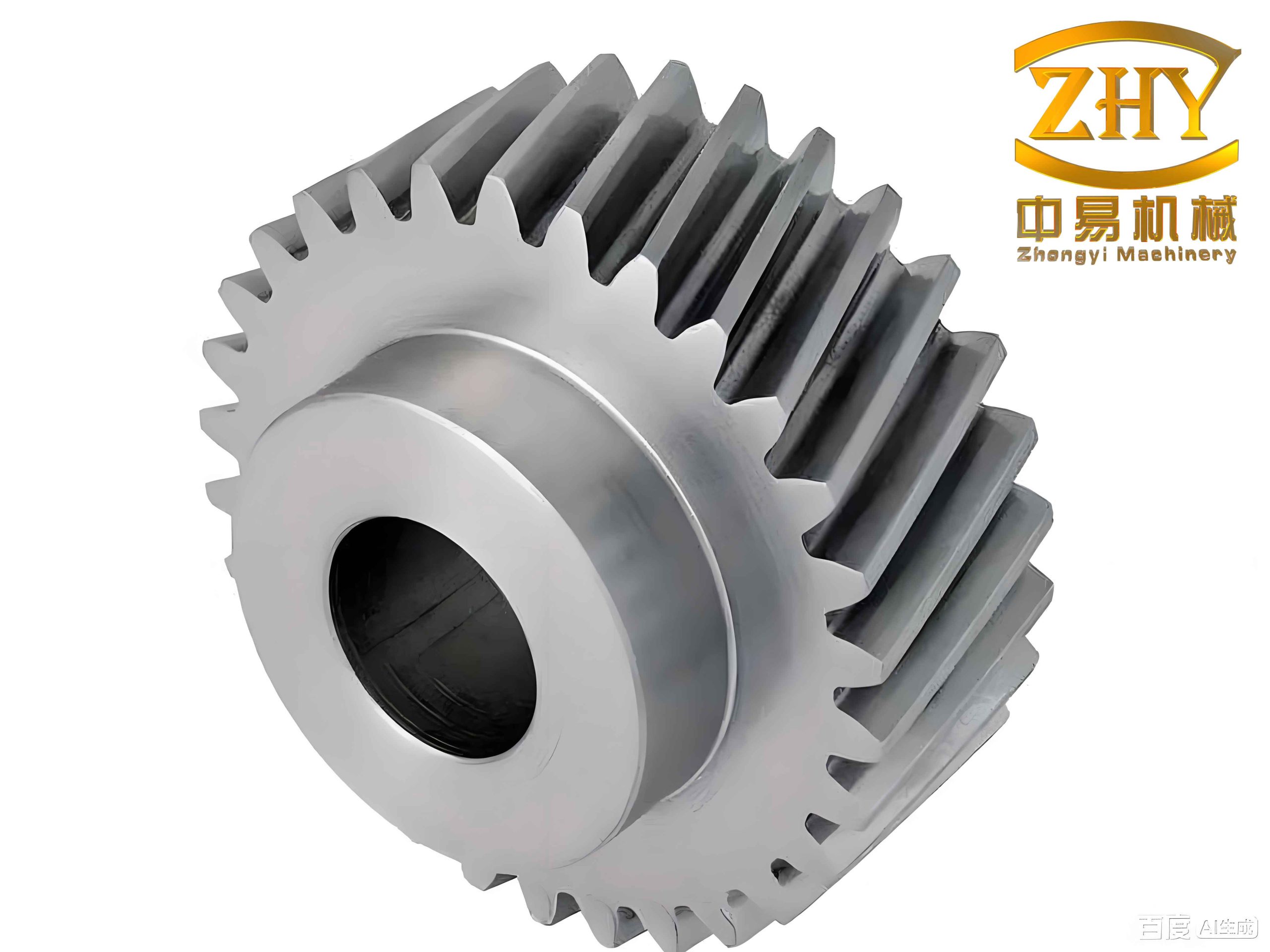
The helical gears studied here had a complex geometry with 65 teeth and eight circular holes. Because the number of teeth is odd and the number of holes is even, the tooth pattern and hole pattern cannot be matched by a simple symmetry condition. Therefore, I modeled the entire helical gear rather than a single tooth sector. This was necessary to capture the global distortion and the interaction between the tooth rim and the web. The main technical requirements after heat treatment were as follows.
| Performance item | Requirement |
|---|---|
| Effective case depth | 0.40 to 0.85 mm |
| Surface hardness | 680 to 850 HV1 |
| Core hardness | 320 to 480 HV1 |
| Surface hardness after grinding | ≥ 650 HV1 |
The helical gears were made of 20CrMnTiH steel. The chemical composition is given in the following table. The alloying elements Cr, Mn, and Si increase hardenability. Ti refines the austenite grain size by forming TiC and TiN particles that pin grain boundaries. This is beneficial for controlling distortion because finer prior austenite grains tend to reduce transformation strain and improve toughness.
| Element | C | Cr | Mn | Ti | Si | P | S | Fe |
|---|---|---|---|---|---|---|---|---|
| Content (wt%) | 0.184 | 1.21 | 0.993 | 0.054 | 0.224 | 0.012 | 0.008 | Balance |
Before heat treatment, the microstructure consisted of fine ferrite and pearlite. The prior austenite grain size was about grade 9, and the ferrite-pearlite banding was rated as B2. Banded structures can cause uneven hardness and local distortion after quenching, so I paid attention to the initial microstructure when interpreting the simulation results. However, the main focus of this work was the carburizing and quenching process itself.
3. Finite Element Model and Mesh Generation
I built the three-dimensional model of the helical gears and exported it in a neutral format for finite element preprocessing. I used hexahedral elements because they provide better accuracy and convergence than tetrahedral elements for coupled heat-treatment problems. To choose an appropriate mesh size, I performed a preliminary study on a cube specimen with edge length 10 mm. I compared carbon concentration profiles for element sizes of 1.5 mm, 1.0 mm, and 0.67 mm. The results showed that when the element size was 1.5 mm, the error was relatively large. When the element size was 1.0 mm or smaller, the carbon profile was essentially the same. Therefore, I set the tooth-flank mesh size to about 0.75 mm to ensure high accuracy while keeping the computation manageable.
| Mesh parameter | Value |
|---|---|
| Element type | Hexahedral |
| Global target size | Approximately 0.75 mm on tooth flanks |
| Total number of elements | 115,430 |
| Total number of nodes | 144,726 |
The boundary conditions included heat-transfer boundaries, carbon-diffusion boundaries, and mechanical constraints. The heat-transfer and carbon-diffusion boundaries were applied to all external surfaces exposed to the furnace atmosphere and quenching oil. For mechanical constraints, I fixed the displacement and rotation in the yz and xz directions at selected points on the cross-section. These constraints prevent rigid-body motion while allowing free distortion of the helical gears during quenching.
| Condition type | Application | Purpose |
|---|---|---|
| Heat-transfer boundary | All exposed surfaces | Exchange heat with furnace and quenchant |
| Carbon-diffusion boundary | All exposed surfaces | Supply carbon from atmosphere |
| Mechanical constraint | Selected points on cross-section | Prevent rigid-body motion |
4. Governing Equations for Multi-Field Coupling
The heat-treatment simulation is based on the coupling of temperature, carbon diffusion, phase transformation, and stress/strain. The material is treated as a mixture of phases. The volume fractions of all phases must sum to unity. I denote the volume fraction of phase I by \(\xi_I\), and the mixture rule is written as follows.
$$ X = \sum_{I=1}^{N} X_I \xi_I , \quad \sum_{I=1}^{N} \xi_I = 1 $$
Here \(X\) can be any mixture property, such as density, thermal conductivity, specific heat, or elastic modulus. The phase fractions change during heating, carburizing, and quenching, so the material properties are updated at every time step.
4.1 Temperature Field
The temperature field controls carbon diffusion and all phase transformations. I used the heat-conduction equation with terms for latent heat and mechanical dissipation. The general form can be written as follows.
$$ \rho c \dot{T} = \nabla \cdot (k \nabla T) + \dot{q}_{\mathrm{latent}} + \dot{q}_{\mathrm{mech}} $$
In this equation, \(\rho\) is density, \(c\) is specific heat, \(k\) is thermal conductivity, \(T\) is temperature, and \(\dot{q}_{\mathrm{latent}}\) represents the latent heat released or absorbed during phase transformation. The mechanical dissipation term \(\dot{q}_{\mathrm{mech}}\) is usually small compared with the latent heat, but I included it for completeness. The boundary condition for heat transfer is expressed as follows.
$$ -k \frac{\partial T}{\partial n} = h_T (T – T_W) $$
Here \(h_T\) is the heat-transfer coefficient, \(T_W\) is the quenchant temperature, and \(n\) is the outward normal direction. For radiation at high temperature, I also considered a radiation boundary condition of the form:
$$ -k \frac{\partial T}{\partial n} = \varepsilon \sigma (T^4 – T_W^4) $$
where \(\varepsilon\) is emissivity and \(\sigma\) is the Stefan-Boltzmann constant. The heat-transfer coefficient of the quenching oil was specified as a function of temperature. The maximum heat-transfer coefficient occurred near 850 K, where the vapor blanket collapses and nucleate boiling begins. This strongly influences the cooling rate of the helical gears.
4.2 Carbon Diffusion
Carbon diffusion is described by Fick’s second law. Because the carbon concentration varies with depth and time, the diffusion equation is solved together with the temperature field.
$$ \frac{\partial C}{\partial t} = \nabla \cdot (D_C \nabla C) $$
The carbon diffusion coefficient \(D_C\) depends on temperature and carbon concentration. The surface boundary condition is given by:
$$ -D_C \frac{\partial C}{\partial n} = \beta_C (C_W – C) $$
where \(\beta_C\) is the surface reaction rate coefficient, \(C_W\) is the carbon potential in the atmosphere, and \(C\) is the carbon concentration at the surface. This boundary condition allows the surface carbon concentration to approach the atmosphere carbon potential. In my process, the carbon potential was controlled in stages to avoid excessive surface carbon and to reduce retained austenite.
4.3 Phase Transformation
For diffusion-controlled transformations such as ferrite, pearlite, and bainite, I used a modified Johnson-Mehl-Avrami equation. The volume fraction of bainite, for example, can be written as:
$$ \xi_B = 1 – \exp\left[-\int_0^t f_1(T) f_2(\sigma_{ij}) f_3(C) (t-\tau)^3 d\tau\right] $$
where \(f_1(T)\) is a temperature function, \(f_2(\sigma_{ij})\) is a stress function, and \(f_3(C)\) is a carbon-concentration function. For martensitic transformation, which is diffusionless, I used the Magee model:
$$ \xi_M = 1 – \exp[-\alpha (M_s – T_q)] $$
In this expression, \(M_s\) is the martensite start temperature, \(T_q\) is the quenchant temperature, and \(\alpha\) is a constant. The martensite start temperature depends on carbon concentration and alloying elements. Because the surface has higher carbon than the core, the surface transforms to martensite at a lower temperature. This difference in transformation timing is a major source of internal stress in carburized helical gears.
4.4 Stress and Strain
The total strain in the helical gears during heat treatment includes elastic strain, plastic strain, thermal strain, transformation expansion strain, and transformation plasticity strain. I used the following additive decomposition:
$$ \varepsilon_{ij} = \varepsilon_{ij}^{e} + \varepsilon_{ij}^{p} + \varepsilon_{ij}^{T} + \varepsilon_{ij}^{m} + \varepsilon_{ij}^{tp} $$
The elastic strain is related to stress by Hooke’s law:
$$ \varepsilon_{ij}^{e} = \frac{1+\nu}{E} \sigma_{ij} – \frac{\nu}{E} \sigma_{kk} \delta_{ij} $$
The thermal strain is given by:
$$ \varepsilon_{ij}^{T} = \alpha (T – T_0) \delta_{ij} $$
where \(\alpha\) is the thermal expansion coefficient and \(T_0\) is the reference temperature. The transformation expansion strain is calculated from the volume change of each phase:
$$ \varepsilon_{ij}^{m} = \sum_{I=1}^{N} \beta_I \xi_I \delta_{ij} $$
Here \(\beta_I\) is the transformation expansion coefficient of phase I. For martensite, \(\beta_I\) is positive and relatively large, which contributes to the compressive stress in the case and tensile stress in the core. The transformation plasticity strain is written as:
$$ \varepsilon_{ij}^{tp} = \sum_{I=1}^{N} k_I \xi_I (1-\xi_I) s_{ij} $$
where \(k_I\) is the transformation plasticity coefficient and \(s_{ij}\) is the deviatoric stress. Transformation plasticity is important because it allows plastic deformation even when the applied stress is below the yield strength. I used temperature-dependent yield functions:
$$ F = f(\sigma_{ij}, \kappa, T) – K(\kappa, T) = 0 $$
where \(\kappa\) is the hardening parameter. The hardening parameter evolves with plastic strain and temperature. The flow stress can be approximated by:
$$ \sigma_y = \sigma_0 + K \varepsilon_p^n $$
where \(\sigma_0\) is the initial yield strength, \(K\) is the hardening coefficient, \(\varepsilon_p\) is the equivalent plastic strain, and \(n\) is the hardening exponent. These equations were solved iteratively at each time step.
4.5 Hardness Model
I estimated hardness from the phase fractions and carbon concentration. Martensite hardness depends mainly on carbon content, while bainite and ferrite-pearlite have lower hardness. The mixture hardness can be expressed as:
$$ H = \sum_{I=1}^{N} H_I \xi_I $$
where \(H_I\) is the hardness of phase I. For martensite, I used a carbon-dependent relation of the form:
$$ H_M = a_0 + a_1 C + a_2 C^2 $$
where \(a_0\), \(a_1\), and \(a_2\) are constants fitted from experimental data. This hardness model allowed me to compare the simulated hardness profile with measured Vickers hardness values.
5. Heat-Treatment Process and Experimental Validation
The heat-treatment cycle I used began with heating to 1168.15 K in a continuous carburizing furnace. The carbon potential was 1.0% during the strong carburizing stage, which lasted 162 min. Then the temperature was reduced to 1158.15 K for the diffusion stage, with a carbon potential of 0.86% for 45 min. After that, the helical gears were cooled to 1108.15 K for equalization, with a carbon potential of 0.76% for 54 min. Finally, the helical gears were oil-quenched to room temperature. The process curve can be summarized as follows.
| Stage | Temperature (K) | Carbon potential (%) | Time (min) |
|---|---|---|---|
| Heating and strong carburizing | 1168.15 | 1.00 | 162 |
| Diffusion | 1158.15 | 0.86 | 45 |
| Equalization before quenching | 1108.15 | 0.76 | 54 |
| Oil quenching | Room temperature | — | Until cooled |
The heat-transfer coefficient of the quenching oil was specified as a function of temperature. The maximum value occurred near 850 K. At temperatures above 900 K, a vapor film forms on the surface and reduces the heat-transfer coefficient. At temperatures below 600 K, convection dominates and the heat-transfer coefficient decreases. The combination of these regimes produces a non-uniform cooling history in the helical gears.
5.1 Carbon Concentration
After carburizing and quenching, the measured surface carbon concentration was about 0.756 wt%, and the carbon concentration decreased gradually with depth. At a depth of about 1.2 mm, the carbon concentration approached the core value of about 0.21 wt%. The effective case depth, defined as the depth where hardness falls to 550 HV1, was about 0.75 mm. The simulated carbon profile agreed well with the measured profile obtained by the layer-removal method. The error was small, which confirmed that the diffusion model and the boundary condition were appropriate.
| Depth (mm) | Measured carbon (wt%) | Simulated carbon (wt%) |
|---|---|---|
| 0.00 | 0.756 | 0.760 |
| 0.20 | 0.680 | 0.690 |
| 0.40 | 0.560 | 0.575 |
| 0.60 | 0.430 | 0.440 |
| 0.80 | 0.330 | 0.335 |
| 1.00 | 0.260 | 0.265 |
| 1.20 | 0.210 | 0.215 |
5.2 Microstructure
The carburized case consisted of fine acicular martensite and a small amount of retained austenite. The prior austenite grain size was fine because the carburizing temperature was moderate and Ti additions inhibited grain growth. The martensite packet size was small, and the microstructure rating was about grade 2. In the transition zone, the microstructure contained both acicular martensite and lath martensite. In the core, the microstructure was mainly low-carbon lath martensite with a small amount of lower bainite.
X-ray diffraction showed that the case was mainly body-centered cubic martensite. The lattice parameter was about 2.886 Å. Retained austenite was not detected by XRD because its content was below the detection limit. Using the Magee equation, I estimated the retained austenite content to be about 2%. The simulated retained austenite content was about 1.2%. These values are reasonably close, considering the uncertainty in the \(M_s\) temperature and the local carbon concentration.
| Region | Main phases | Morphology | Notes |
|---|---|---|---|
| Case | Acicular martensite + retained austenite | Fine needle-like | High hardness, high carbon |
| Transition | Acicular martensite + lath martensite | Mixed | Hardness decreases with depth |
| Core | Low-carbon lath martensite + lower bainite | Lath and bainitic | Higher toughness |
5.3 Hardness
The measured surface hardness reached about 778 HV1, and the core hardness was about 355 HV1. The simulated surface hardness was about 741 to 745 HV1. The difference between measured and simulated surface hardness was about 35 HV1, which is within 5%. This difference is acceptable because the measured indentation samples a small local region, while the simulated value represents an average over a larger area. The effective case depth, defined by the 550 HV1 threshold, was about 0.75 mm in both measurement and simulation.
| Position | Measured hardness (HV1) | Simulated hardness (HV1) | Difference (%) |
|---|---|---|---|
| Surface L1 | 778 | 743 | 4.5 |
| Surface L2 | 772 | 742 | 3.9 |
| Surface L3 | 770 | 741 | 3.8 |
| Core | 355 | 360 | 1.4 |
5.4 Distortion and Helix Total Deviation
Distortion is one of the most important quality indices for helical gears. I measured the displacement of the tooth flanks at the pitch circle and calculated the helix total deviation \(F_\beta\). The maximum simulated distortion was about 90.8 μm at the top of the gear end face, while the minimum distortion was about 1.93 μm. Along the helix direction, the distortion first decreased and then increased. The simulated helix total deviation was about 15 μm on average, and the measured value was also about 15 μm on average. The agreement was good.
| Tooth number | Simulated distortion (μm) | Simulated \(F_\beta\) (μm) | Measured \(F_\beta\) (μm) |
|---|---|---|---|
| 1 | 49.61 | 17.26 | 7.2 |
| 18 | 47.34 | 11.00 | 11.9 |
| 34 | 43.10 | 6.30 | 5.1 |
| 50 | 50.70 | 24.30 | 36.9 |
I also examined the temperature history during quenching. The temperature difference between the tooth flank and the end face reached about 50 K at the early stage of quenching. This difference caused non-uniform thermal stress and transformation stress. The outer end face lost heat faster because the vapor film broke earlier, while the inner region cooled more slowly. This non-uniform cooling is the main reason for the non-uniform distortion of the helical gears.
6. Parametric Study of Carburizing and Quenching
After validating the model, I performed a parametric study. The variables were strong carburizing time, diffusion time, carburizing temperature, and cooling rate. I evaluated carbon concentration, case depth, martensite fraction, retained austenite fraction, surface hardness, distortion, and helix total deviation \(F_\beta\).
6.1 Effect of Holding Time
I selected three levels of strong carburizing time (132, 162, and 212 min) and three levels of diffusion time (30, 45, and 60 min). The results showed that increasing both times increases the case depth. The strong carburizing time had a slightly larger effect than the diffusion time. The case depth ranged from about 0.63 mm to 0.82 mm. The carbon profile became smoother as the total holding time increased. The martensite content and surface hardness increased slightly with longer holding time, but the change was small. The retained austenite content decreased slightly. Distortion varied with holding time, but the distribution pattern along the helix remained similar. The maximum distortion was about 49.24 μm, and the minimum was about 43.30 μm. The helix total deviation ranged from about 12.1 to 15.3 μm.
| Strong time (min) | Diffusion time (min) | Case depth (mm) | Martensite (wt%) | Hardness (HV1) | Distortion (μm) | \(F_\beta\) (μm) |
|---|---|---|---|---|---|---|
| 132 | 30 | 0.63 | 98.515 | 741.4 | 45.58 | 13.23 |
| 132 | 45 | 0.67 | 98.580 | 742.0 | 44.78 | 14.56 |
| 132 | 60 | 0.70 | 98.625 | 741.0 | 49.26 | 15.30 |
| 162 | 30 | 0.69 | 98.767 | 742.0 | 49.24 | 14.91 |
| 162 | 45 | 0.72 | 98.783 | 743.0 | 47.40 | 14.70 |
| 162 | 60 | 0.73 | 98.812 | 741.9 | 45.03 | 13.97 |
| 212 | 30 | 0.78 | 98.884 | 743.0 | 46.50 | 13.91 |
| 212 | 45 | 0.80 | 98.904 | 744.6 | 45.00 | 13.13 |
| 212 | 60 | 0.82 | 98.927 | 745.5 | 43.30 | 12.10 |
6.2 Effect of Carburizing Temperature
I studied carburizing temperatures of 885, 895, 900, 910, and 920 °C. The carbon concentration profile became smoother as temperature increased because carbon diffusion is faster at higher temperature. The case depth increased from about 0.72 mm at 885 °C to about 0.77 mm at 920 °C. However, the surface martensite content and hardness did not change much. The martensite content was about 98.76 wt%, and the retained austenite content was about 1.24 wt%. The surface hardness remained around 743 HV1. The distortion, however, varied with carburizing temperature. The minimum distortion and minimum \(F_\beta\) occurred at 910 °C. This indicates that there is an optimal carburizing temperature for minimizing distortion: it must be high enough to provide sufficient carbon diffusion but not so high that austenite grain growth and thermal gradients become excessive.
| Carburizing temperature (°C) | Case depth (mm) | Martensite (wt%) | Hardness (HV1) | Distortion (μm) | \(F_\beta\) (μm) |
|---|---|---|---|---|---|
| 885 | 0.72 | 98.763 | 743.0 | 42.46 | 11.51 |
| 895 | 0.73 | 98.763 | 743.0 | 47.40 | 14.70 |
| 900 | 0.73 | 98.763 | 743.0 | 43.63 | 12.57 |
| 910 | 0.74 | 98.763 | 743.0 | 39.17 | 10.18 |
| 920 | 0.77 | 98.815 | 743.5 | 45.62 | 13.68 |
6.3 Effect of Cooling Rate
The cooling rate was controlled by the heat-transfer coefficient of the quenching oil. I tested five heat-transfer coefficient curves, labeled H1 through H5. H2 and H3 were lower than H1, while H4 and H5 were higher. The carbon concentration profile did not change with cooling rate, as expected, because carbon diffusion occurs mainly at high temperature before quenching. The martensite content and hardness, however, depended strongly on cooling rate. Faster cooling produced more martensite and higher hardness. H4 gave the highest hardness, about 745.7 HV1, while H3 gave the lowest, about 728.9 HV1. The retained austenite content was higher for slower cooling.
The effect of cooling rate on distortion was even more pronounced. H2 and H3 produced large distortion and large helix total deviation. H4 produced the smallest distortion and \(F_\beta\). The distortion for H4 was about 42.24 μm, and \(F_\beta\) was about 8.66 μm. For H3, the distortion reached about 69.12 μm and \(F_\beta\) reached about 58.91 μm. This shows that cooling rate is the most influential parameter for distortion control. A properly selected cooling rate can reduce thermal gradients and transformation gradients, leading to more uniform distortion.
| Cooling case | Martensite (wt%) | Retained austenite (wt%) | Hardness (HV1) | Distortion (μm) | \(F_\beta\) (μm) |
|---|---|---|---|---|---|
| H1 | 98.763 | 1.237 | 743.0 | 47.40 | 14.70 |
| H2 | 96.737 | 3.263 | 736.5 | 74.30 | 54.00 |
| H3 | 97.734 | 2.266 | 728.9 | 69.12 | 58.91 |
| H4 | 98.886 | 1.114 | 745.7 | 42.24 | 8.66 |
| H5 | 98.756 | 1.244 | 745.3 | 53.88 | 23.70 |
7. Process Optimization by Orthogonal Experiments
To identify the most influential parameters and the best combination, I designed an orthogonal experiment with four factors and three levels. The factors were carburizing temperature, strong carburizing time, diffusion time, and cooling rate. The levels are listed in the following table.
| Level | Carburizing temperature (°C) | Strong time (min) | Diffusion time (min) | Cooling rate |
|---|---|---|---|---|
| 1 | 885 | 132 | 30 | H1 |
| 2 | 895 | 162 | 45 | H4 |
| 3 | 910 | 192 | 60 | H5 |
I ran nine simulations according to the orthogonal array. The results are shown below. The distortion ranged from about 39 to 55 μm, and the helix total deviation ranged from about 8 to 27 μm. All combinations satisfied the hardness and case-depth requirements.
| Run | Carburizing temperature (°C) | Strong time (min) | Diffusion time (min) | Cooling rate | Distortion (μm) | \(F_\beta\) (μm) |
|---|---|---|---|---|---|---|
| 1 | 885 | 132 | 30 | H1 | 42.21 | 14.85 |
| 2 | 895 | 132 | 45 | H4 | 40.71 | 8.26 |
| 3 | 910 | 132 | 60 | H5 | 49.15 | 23.12 |
| 4 | 910 | 162 | 30 | H4 | 39.45 | 8.17 |
| 5 | 885 | 162 | 45 | H5 | 50.78 | 26.62 |
| 6 | 895 | 162 | 60 | H1 | 45.03 | 13.97 |
| 7 | 895 | 212 | 30 | H5 | 53.61 | 26.25 |
| 8 | 910 | 212 | 45 | H1 | 41.87 | 13.77 |
| 9 | 885 | 212 | 60 | H4 | 39.11 | 9.23 |
I performed range analysis on the results. The range \(R\) for each factor is the difference between the maximum and minimum average response at different levels. A larger \(R\) means that the factor has a stronger effect on the performance index. For both distortion and helix total deviation, the cooling rate had the largest range, followed by carburizing temperature, strong carburizing time, and diffusion time. The order was:
$$ R_D > R_A > R_B > R_C $$
where \(A\) is carburizing temperature, \(B\) is strong time, \(C\) is diffusion time, and \(D\) is cooling rate. The optimal combination from the orthogonal analysis was A3 B1 C3 D2, which corresponds to a carburizing temperature of 910 °C, a strong time of 132 min, a diffusion time of 60 min, and cooling rate H4.
| Index | A: Carburizing temperature | B: Strong time | C: Diffusion time | D: Cooling rate |
|---|---|---|---|---|
| K1 for \(F_\beta\) | 16.90 | 15.41 | 16.42 | 14.20 |
| K2 for \(F_\beta\) | 16.16 | 16.25 | 16.22 | 8.55 |
| K3 for \(F_\beta\) | 15.02 | 16.42 | 15.44 | 25.33 |
| Range \(R\) for \(F_\beta\) | 1.88 | 1.10 | 0.98 | 17.77 |
| K1 for distortion | 44.03 | 44.02 | 45.09 | 43.03 |
| K2 for distortion | 46.45 | 45.09 | 44.45 | 39.76 |
| K3 for distortion | 43.49 | 44.86 | 44.43 | 51.18 |
| Range \(R\) for distortion | 2.96 | 1.06 | 0.66 | 11.42 |
8. Process Optimization by BP Neural Network
Although orthogonal experiments are efficient, they only sample a limited number of discrete combinations. To explore the process window more thoroughly, I built a BP neural network model. The network had four inputs: carburizing temperature, strong carburizing time, diffusion time, and cooling rate. It had two outputs: distortion and helix total deviation \(F_\beta\). I used a three-layer architecture with 15 neurons in the hidden layer, giving a 4-15-2 topology. The input data were normalized using the min-max method:
$$ f = \frac{x – x_{\min}}{x_{\max} – x_{\min}} $$
The training function was trainlm, the hidden-layer transfer function was tansig, and the output-layer transfer function was purelin. I used 36 data sets from simulation and experiment. Of these, 29 were used for training and 7 for testing. The expected error was set to \(1 \times 10^{-4}\), and the learning rate was set to \(9 \times 10^{-2}\). The network converged after 1200 iterations, and the training curve was smooth.
| Network parameter | Value |
|---|---|
| Input neurons | 4 |
| Hidden neurons | 15 |
| Output neurons | 2 |
| Training function | trainlm |
| Hidden transfer function | tansig |
| Output transfer function | purelin |
| Learning rate | 0.09 |
| Target error | \(1 \times 10^{-4}\) |
The prediction performance of the BP network was evaluated using relative error:
$$ \text{Relative error} = \frac{\text{Predicted value} – \text{Measured value}}{\text{Measured value}} \times 100\% $$
The average relative error for distortion was about 4.1%, and the average relative error for helix total deviation was about 3.8%. Most errors were below 5%. This indicates that the BP neural network had good generalization ability and could accurately map the relationship between process parameters and final helical gear performance.
| Test sample | Distortion error (%) | \(F_\beta\) error (%) |
|---|---|---|
| 1 | 3.9 | 3.5 |
| 2 | 4.4 | 4.1 |
| 3 | 3.7 | 3.9 |
| 4 | 4.8 | 4.3 |
| 5 | 4.2 | 3.6 |
| 6 | 3.8 | 3.4 |
| 7 | 4.0 | 3.8 |
Using the trained BP network, I searched the process space and found an optimal combination: carburizing temperature 915 °C, strong carburizing time 150 min, diffusion time 40 min, and cooling rate H4. I then verified this combination with COSMAP. The predicted distortion was 36.72 μm, and the simulated distortion was 38.91 μm. The predicted \(F_\beta\) was 7.89 μm, and the simulated \(F_\beta\) was 8.13 μm. The relative errors were within 5%, which confirmed the reliability of the BP optimization.
| Method | Distortion (μm) | \(F_\beta\) (μm) |
|---|---|---|
| BP network prediction | 36.72 | 7.89 |
| COSMAP simulation | 38.91 | 8.13 |
| Relative error | 5.6% | 3.0% |
9. Discussion
The results show that the coupled multi-field model can reproduce the main features of carburizing and quenching for complex helical gears. Carbon diffusion is controlled by temperature and time, and the case depth increases with both. However, longer holding times also increase the total thermal exposure, which can modify distortion. Carburizing temperature has a dual effect: higher temperature accelerates diffusion and increases case depth, but it also increases the thermal gradient and may coarsen austenite grains. In my simulations, 910 °C gave the best combination of case depth and low distortion in the orthogonal study, while the BP network suggested 915 °C as the optimum when strong time and diffusion time were adjusted. The difference is small and reflects the fact that the optimum is a broad region rather than a single sharp point.
The cooling rate is the dominant factor for distortion. When the cooling rate is too low, the vapor film lasts longer and cooling becomes non-uniform. The helical gears may then experience uneven transformation and larger helix deviation. When the cooling rate is too high, thermal gradients become steep, and thermal stress can also increase distortion. The best result occurred at an intermediate-high cooling rate, labeled H4. This is consistent with the idea that a balanced cooling path can minimize the combined effects of thermal stress and transformation stress.
For helical gears, distortion is not uniform along the tooth width. The temperature history at the end faces differs from that at the mid-section. The end faces cool faster, while the central region cools more slowly. This causes the helix to twist and the pitch to shift. The helix total deviation \(F_\beta\) is therefore a useful integrated measure of distortion. My model predicted the same general trend as the measurements, although there were local differences due to banded microstructure, residual stress from machining, and fixture effects.
The BP neural network provided a flexible way to optimize the process. Unlike orthogonal experiments, which evaluate only a fixed set of levels, the neural network can interpolate between points and predict performance for untested combinations. The 4-15-2 network had enough capacity to capture the nonlinear relationship between process parameters and performance. The relative errors were small, and the comparison with COSMAP confirmed the network’s practical value. This approach can reduce the number of physical trials needed to optimize carburizing and quenching for helical gears.
10. Practical Implications
From an industrial point of view, the results suggest several practical rules for carburizing and quenching helical gears. First, the cooling rate should be selected carefully. It is not always best to use the fastest quench. An intermediate-high cooling rate with a well-designed oil and agitation pattern can reduce helix deviation while still achieving the required hardness. Second, the carburizing temperature should be high enough to achieve the specified case depth within a reasonable time, but not so high that grain growth and thermal distortion increase. Third, the strong carburizing time and diffusion time should be balanced. A longer diffusion stage can smooth the carbon profile and reduce retained austenite, but excessive time may not improve performance further and may increase distortion. Fourth, the initial microstructure should be controlled. Banded ferrite-pearlite can cause local hard spots and non-uniform transformation, which increases distortion.
I also found that simulation can be used to define the process window before physical trials. The model can predict carbon profiles, hardness, phase fractions, and distortion for a wide range of conditions. The BP network can then be used as a fast surrogate model for optimization. This two-step approach is efficient and can be applied to other helical gears with different geometries and materials.
11. Limitations and Future Work
The model I developed has several limitations. The material properties were taken from a combination of database values and literature data, so there may be some uncertainty in the transformation plasticity coefficients and heat-transfer coefficients. The quenching oil heat-transfer coefficient was specified as a function of temperature, but in reality it also depends on agitation, part orientation, and surface condition. The initial residual stress from machining was not included. The banded microstructure was not explicitly represented in the finite element model. These factors can influence local distortion.
Future work could include measuring the heat-transfer coefficient directly for the actual quench tank and fixture. It could also include a microstructure-based model that accounts for banding and inclusion distribution. The BP network could be improved by adding more training data from experiments and by using a genetic algorithm or particle swarm optimization to search the process space more efficiently. Finally, the optimized process should be validated in production trials with multiple helical gears to confirm statistical reproducibility.
12. Conclusions
I studied the carburizing and quenching of complex helical gears made of 20CrMnTiH steel using a coupled multi-field finite element model and experimental validation. The main conclusions are as follows.
1. The coupled temperature-diffusion-phase-stress model predicted carbon concentration, case depth, microstructure, hardness, and distortion with good accuracy. The measured surface carbon was about 0.756 wt%, the surface hardness was about 778 HV1, the effective case depth was about 0.75 mm, and the helix total deviation was about 14.7 μm. These values agreed with the simulation.
2. The case microstructure consisted of fine acicular martensite and a small amount of retained austenite. The transition zone contained mixed acicular and lath martensite. The core contained low-carbon lath martensite and a small amount of lower bainite. The fine grain size was attributed to moderate carburizing temperature and Ti microalloying.
3. Carbon concentration and case depth increased with carburizing temperature and holding time. Strong carburizing time had a slightly larger effect on case depth than diffusion time. Surface martensite content and hardness increased slightly with longer holding time, but carburizing temperature had little effect on surface hardness.
4. Cooling rate was the most influential parameter for distortion and helix total deviation. The best cooling rate in this study was H4, which gave the smallest distortion and \(F_\beta\). The order of influence was cooling rate > carburizing temperature > strong time > diffusion time.
5. Orthogonal experiments identified the optimal combination as 910 °C carburizing temperature, 132 min strong time, 60 min diffusion time, and cooling rate H4. The BP neural network identified 915 °C, 150 min strong time, 40 min diffusion time, and cooling rate H4. The BP prediction was verified by COSMAP with errors within 5%.
6. The combination of finite element simulation and BP neural network optimization provides a practical method for designing carburizing and quenching processes for helical gears. It reduces the need for trial-and-error experiments and helps control distortion while maintaining the required hardness and case depth.
Overall, this work shows that accurate multi-field simulation and intelligent optimization can be used together to improve the heat-treatment quality of helical gears for electric vehicles. The methods and findings can be extended to other case-hardened components where distortion control is critical.