
I have developed a comprehensive on-machine measurement strategy for face gear grinding using a worm grinding wheel machine. The face gear transmission is a reliable and smooth solution for intersecting axes, and its machining accuracy directly determines performance. Accurate tooth surface error measurement can guide subsequent corrective machining. However, conventional offline measurement using coordinate measuring machines or gear measuring instruments introduces installation errors due to repeated loading and unloading. Therefore, I focused on on-machine measurement of face gear. During on-machine measurement, the probe pre-travel error significantly affects tooth surface accuracy. I established a prediction model for the comprehensive pre-travel error based on a PSO-CNN neural network, and I proposed a precise tooth surface matching method to obtain accurate face gear errors. The experimental results demonstrate that the left tooth surface accuracy improved by 61.33% and the right tooth surface accuracy improved by 71.15%. The on-machine measurement results are basically consistent with those obtained from a Klingelnberg measuring instrument, satisfying the face gear on-machine measurement accuracy requirements.
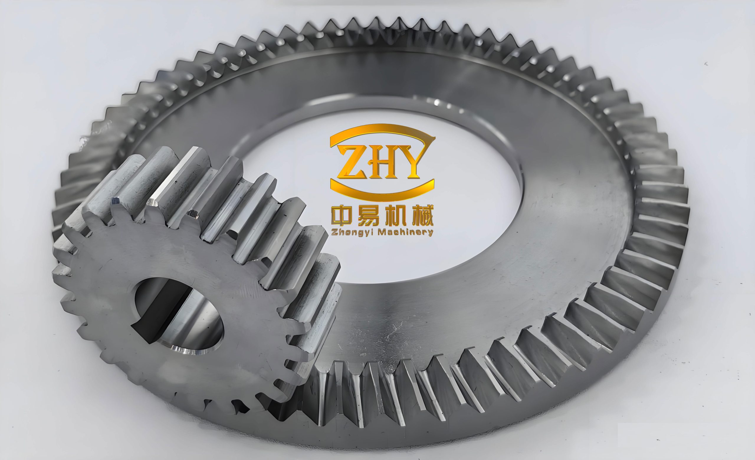
1. Mathematical Model of the Face Gear Tooth Surface
I constructed a face gear tooth surface model based on the two-parameter envelope principle to provide a standard comparison model for on-machine measurement. Considering the tooth surface characteristics and machining method, I first established the worm grinding wheel profile using conjugate surface envelope theory. Then, I solved the tooth surface equation through the two-parameter envelope principle and planned the theoretical measurement grid.
According to the envelope principle, the worm grinding wheel profile equation is expressed as:
$$ r_w(\theta_s,\phi_s) = r_w(\phi_s,\theta_s,u_s(\phi_s,\theta_s)) \tag{1} $$
where $\theta_s$ is the angle parameter of the involute, $u_s$ is the tooth width direction parameter, and the relationship between the grinding wheel rotation angle $\phi_w$ and the generating gear rotation angle $\phi_s$ is given by $\phi_w = m_{ws}\phi_s$, where $m_{ws}$ is the transmission ratio between the generating gear and the worm grinding wheel.
I defined the face gear model and the generating gear model to have the same origin height, with $H_2$ being the distance from the face gear model origin to the face gear tooth tip in the Z direction. The coordinate systems are defined as follows: $O_w – X_wY_wZ_w$ is the worm rotation coordinate system, $O_4 – X_4Y_4Z_4$ is a translation coordinate system at a distance $H_1$ from the face gear origin, $O_5 – X_5Y_5Z_5$ and $O_6 – X_6Y_6Z_6$ are auxiliary coordinate systems, $O_7 – X_7Y_7Z_7$ is the initial position coordinate system of the face gear, $O_c – X_cY_cZ_c$ is the face gear rotation coordinate system, and $O_d – X_dY_dZ_d$ is the design coordinate system based on the face gear tooth tip.
During transmission, the rotation angles $\Delta_e$ and $\Delta_d$ satisfy the following transmission ratio relationship:
$$ \Delta_d = m_{dw}\Delta_e = \frac{N_w}{N_d}\Delta_e \tag{2} $$
where $m_{dw}$ is the transmission ratio between the face gear and the worm grinding wheel, $N_w$ is the number of worm starts, and $N_d$ is the number of face gear teeth. The coordinate transformation matrix $M_{dw}$ from the worm rotation coordinate system to the design coordinate system is:
$$ M_{dw}(\Delta_e,\Delta_L) = M_{dc}M_{c7}M_{76}M_{65}M_{54}M_{4w} = \begin{bmatrix}
-\cos(\Delta_d+\lambda)\cos(\Delta_e) & \cos(\Delta_d+\lambda)\sin(\Delta_e) & \sin(\Delta_d+\lambda) & \Delta_L\cos(\Delta_d) \\
\sin(\Delta_d+\lambda)\cos(\Delta_e) & -\sin(\Delta_d+\lambda)\sin(\Delta_e) & \cos(\Delta_d+\lambda) & -\Delta_L\sin(\Delta_d) \\
\sin(\Delta_e) & \cos(\Delta_e) & 0 & H_1+H_2 \\
0 & 0 & 0 & 1
\end{bmatrix} \tag{3} $$
According to the two-parameter envelope principle, the face gear equation is obtained as:
$$ r_d(\theta_s,\phi_s,\Delta_e,\Delta_L) = M_{dw}(\Delta_e,\Delta_L) r_w(\theta_s,\phi_s) \tag{4} $$
I established two independent meshing equations for the two parameters:
$$ \left( \frac{\partial r_d}{\partial \theta_s} \times \frac{\partial r_d}{\partial \phi_s} \right) \cdot \frac{\partial r_d}{\partial \Delta_e} = 0 \tag{5} $$
$$ \left( \frac{\partial r_d}{\partial \theta_s} \times \frac{\partial r_d}{\partial \phi_s} \right) \cdot \frac{\partial r_d}{\partial \Delta_L} = 0 \tag{6} $$
where $\frac{\partial r_d}{\partial \theta_s} \times \frac{\partial r_d}{\partial \phi_s}$ is the normal vector at the meshing point between the worm grinding wheel and the face gear, $\frac{\partial r_d}{\partial \Delta_e}$ is the relative velocity along the worm grinding wheel feed direction, and $\frac{\partial r_d}{\partial \Delta_L}$ is the relative velocity along the face gear rotation direction. The basic parameters of the face gear are listed in Table 1.
| Parameter | Value | Parameter | Value |
|---|---|---|---|
| Face gear tooth number | 48 | Pinion cutter tooth number | 23 |
| Face gear module | 3.9 | Pressure angle (°) | 25 |
| Addendum coefficient | 1 | Dedendum coefficient | 1 |
| Clearance coefficient | 0.25 | Inner radius (mm) | 90 |
| Outer radius (mm) | 100 | Pinion cutter module | 3.9 |
By eliminating $\phi_s$ and $\Delta_e$ while keeping $\theta_s$ constant and varying $\Delta_L$, I obtained the face gear tooth longitudinal line. By keeping $\Delta_L$ constant and varying $\theta_s$, I obtained the face gear tooth profile line. According to the bevel gear measurement grid standard and the tooth surface characteristics, I set the upper and lower boundaries by contracting 5% of the difference between the tangent value of $\theta_{s1}$ corresponding to the tooth tip point at the outer circle and the tangent value of $\theta_{s2}$ corresponding to the transition curve point. I divided the tangent value of $\theta_s$ into 4 equal parts. At the same time, I set the front and rear boundaries by taking 10% of the difference between the inner and outer radii and divided them into 8 equal parts. Thus, I obtained the theoretical measurement grid shown in the model. Let the theoretical tooth surface coordinates be $r_d = [x_d\ y_d\ z_d\ 1]^T$ and the normal vector at each point be $n_d = [n_{xd}\ n_{yd}\ n_{zd}\ 1]^T$.
2. On-Machine Measurement Strategy Based on the Worm Grinding Wheel Machine
I designed a complete on-machine measurement flow for face gear. The first step is to calibrate the probe radius using a standard sphere and to model the comprehensive pre-travel error. The second step is to perform plane reference calibration to determine the Z-direction measurement reference. The third step is to perform roundness calibration of the face gear outer circle to determine the center coordinates of the face gear measurement coordinate system. The fourth step is to perform tooth slot alignment to roughly match the design tooth surface with the actual tooth surface and establish the measurement coordinate system. The fifth step is to plan the measurement path according to the calculated measurement point coordinates, measure the tooth surface, and obtain the tooth surface error through precise tooth surface matching.
On-machine measurement obtains coordinates in the machine tool coordinate system, but the calculated theoretical points are in the design coordinate system. Therefore, I transformed the design coordinate system coordinates into the machine tool coordinate system to control the probe for measurement and obtain the probe center coordinates in the machine tool coordinate system. The transformation from the design coordinate system to the machine tool coordinate system is described as follows. In actual measurement, the touch-trigger probe is installed on the Y-axis, and the face gear is fixed on the C-axis rotary table.
The translation matrix and rotation matrix from the design coordinate system to the machine tool coordinate system are:
$$ M_{ba} = \begin{bmatrix}
1 & 0 & 0 & D_x \\
0 & 1 & 0 & D_y \\
0 & 0 & 1 & D_z \\
0 & 0 & 0 & 1
\end{bmatrix} \tag{7} $$
$$ M_{nb} = \begin{bmatrix}
\cos C & \sin C & 0 & 0 \\
-\sin C & \cos C & 0 & 0 \\
0 & 0 & 1 & 0 \\
0 & 0 & 0 & 1
\end{bmatrix} \tag{8} $$
The theoretical coordinates and normal vectors of each measurement point on the tooth surface in the machine tool coordinate system are:
$$ \begin{bmatrix} x_b \\ y_b \\ z_b \\ 1 \end{bmatrix} = (M_{nb})^{-1} (M_{ba})^{-1} r_d \tag{9} $$
$$ \begin{bmatrix} n_{xb} \\ n_{yb} \\ n_{zb} \\ 1 \end{bmatrix} = (M_{nb})^{-1} (M_{ba})^{-1} n_d \tag{10} $$
Similarly, the theoretical position and normal vector of the probe sphere center in the machine tool coordinate system can be calculated as:
$$ \begin{bmatrix} x_p \\ y_p \\ z_p \\ 1 \end{bmatrix} = \begin{bmatrix} x_b \\ y_b \\ z_b \\ 1 \end{bmatrix} + R \begin{bmatrix} n_{xb} \\ n_{yb} \\ n_{zb} \\ 1 \end{bmatrix} \tag{11} $$
$$ \begin{bmatrix} n_{xp} \\ n_{yp} \\ n_{zp} \\ 1 \end{bmatrix} = \begin{bmatrix} n_{xb} \\ n_{yb} \\ n_{zb} \\ 1 \end{bmatrix} \tag{12} $$
Based on the calculated theoretical measurement point coordinates and normal vectors, I completed the measurement of the tooth surface elements. First, I calculated the offsets $D_x$, $D_y$, and $D_z$. I controlled the probe to extract a certain number of points on the face gear tooth tip, fitted the best plane using the least squares method to obtain $D_z$. Similarly, I extracted a certain number of points on the face gear outer circumference, fitted a circle to determine $D_x$ and $D_y$.
Finally, I performed tooth slot alignment to obtain the angle $C$ and complete the rough matching between the design tooth surface and the actual tooth surface, establishing the measurement coordinate system. The specific process is as follows:
- First, the probe sphere center reaches $(x_1+i, 0, z_1)$, where $i=1,2,\dots,9$, $z_1$ is set as the machine tool coordinate system position of the tooth surface center point, and $x_1$ is the corresponding X-axis coordinate when the face gear radius is 90 mm. I slowly rotated the face gear C-axis to touch the probe, which emitted a pulse signal, and obtained the positive rotation amount $C_{1i}$. I repeated the same procedure by rotating the C-axis in the opposite direction to obtain the negative rotation amount $C_{2i}$. I recorded the initial value as $C_i = (C_{1i}+C_{2i})/2$ and rotated the C-axis to $C_i$.
- I moved the probe to the next point and repeated step 1 to obtain the rotation amounts $C_{12}$ and $C_{22}$. Then I set $C_i = \sum (C_{1i}+C_{2i})/(2i)$.
- I set a threshold value $e$. If $C_{i+1}-C_i$ is less than $e$, the program stops and the tooth slot alignment is completed, marking the end of rough tooth surface matching.
3. Comprehensive Pre-Travel Error Modeling and Compensation Method
To comprehensively consider the influence of pre-travel error on tooth surface accuracy during face gear on-machine measurement, I used multiple error influencing factors as inputs and the comprehensive pre-travel error of the probe as output. I constructed a comprehensive pre-travel error prediction model based on a PSO-CNN neural network to complete error compensation.
I established an on-machine inspection model for the YS7232 worm grinding wheel machine. The on-machine inspection principle is as follows. First, I measure according to the NC macro program written for the measurement path. Second, the probe touches the tooth surface along the normal direction at a certain speed, and when the preset trigger force is reached, a pulse signal is emitted to obtain the measurement point coordinates. Finally, the NC system acquires the signal and controls the motion axis to stop the measurement.
In actual on-machine measurement, the comprehensive pre-travel error can be divided into the axial pre-travel error $E_{rL}^{\phi}$ and the radial pre-travel error $E_{vs}^{\Delta t \theta}$. The sum of the two gives the comprehensive pre-travel error $E_{vs\Delta t\theta}^{rL\phi}$. The worm grinding wheel machine used in this experiment is an experimental platform, and I used a standard sphere for calibration. Due to the influence of factors such as measurement speed $v$, distance between the positioning point and the measurement point $s$, probe sphere radius $r$, signal delay time $\Delta t$, measurement longitude $\theta$, measurement latitude $\phi$, and stylus length $L$, the comprehensive pre-travel error exhibits nonlinear variation. I constructed a comprehensive pre-travel error model including the above factors for compensation to improve face gear measurement accuracy. According to the on-machine measurement mechanism of the YS7232 worm grinding wheel machine, I used $v$, $s$, $\Delta t$, $\theta$, $\phi$, $L$, and $r$ as input nodes and $E_{vs\Delta t\theta}^{rL\phi}$ as the output node to establish a PSO-CNN based comprehensive pre-travel error prediction model.
3.1 Probe Calibration
To ensure the correctness of $E_{vs\Delta t\theta}^{rL\phi}$, I performed probe radius compensation. The calibration steps are as follows. First, I installed a standard sphere at a suitable position on the NC machine tool, rotated the magnetic base to attach it to the machine tool, and ensured the base was parallel to the machine tool XOY plane. Second, I moved the probe to the initial positioning point near the top of the standard sphere and uniformly took four points along the circumference direction at $\theta=0^\circ$ to determine the approximate sphere center position $(X_0,Y_0,Z_0)$. Third, based on the center position, I set the measurement point coordinates as $(X_Q,Y_Q,Z_Q)$, where $X_Q = X_0 + R\cos\phi\cos\theta$, $Y_Q = Y_0 + R\cos\phi\sin\theta$, and $Z_Q = Z_0 + R\sin\phi$. Fourth, I set the measurement longitude and latitude angle intervals and repeated the third step to obtain all calibration point coordinates. I used the least squares method to fit the sphere and obtain the actual probe radius.
Based on the measured actual coordinates $(x_i,y_i,z_i)$, the theoretical measurement point coordinates satisfy:
$$ (x-a)^2 + (y-b)^2 + (z-c)^2 = R^2 \tag{13} $$
Because there are deviations during measurement, the residual equation is:
$$ \delta(a,b,c,R) = \sum_{i=1}^{n} \left[ (x_i-a)^2 + (y_i-b)^2 + (z_i-c)^2 – R^2 \right]^2 \tag{14} $$
By taking partial derivatives of the deviation:
$$ \frac{\partial \delta(a,b,c,R)}{\partial a} = 0, \quad
\frac{\partial \delta(a,b,c,R)}{\partial b} = 0, \quad
\frac{\partial \delta(a,b,c,R)}{\partial c} = 0, \quad
\frac{\partial \delta(a,b,c,R)}{\partial R} = 0 \tag{15} $$
I obtained the sphere center coordinates $(a,b,c)$ and the fitted sphere radius $R$ of the probe sphere center. Because the standard sphere precision is much higher than the probe precision, the actual probe radius is $r’ = R – R_{\text{standard}}$, where $R_{\text{standard}}$ is the theoretical radius of the standard sphere.
3.2 Radial Pre-Travel Error Model $E_{vs}^{\Delta t \theta}$
Based on the on-machine measurement model of the YS7232 worm grinding wheel machine, I established a radial pre-travel error model $E_{vs}^{\Delta t \theta}$ for the vertical stylus. During measurement, the measurement latitude $\phi$ is always $0^\circ$. When the radial theoretical trigger force $F_1$ of the stylus is reached, the coordinate signal is obtained. Along the longitude measurement direction, only the machine tool X-axis, Y-axis, and Z-axis are required for linkage measurement. First, I initialized the positions of all machine axes and set the A-axis to $0^\circ$. Second, I moved the probe center height to the position where the standard sphere latitude $\phi$ is $0^\circ$. Third, I divided the circumference into $n$ measurement points according to longitude, set the distance between the positioning point and the measurement point as $s$, measured along the normal direction at a constant speed $v$, and obtained the radial position offset $\Delta r$ of the stylus. Finally, I repeated steps 2 and 3 and set multiple measurement speeds for comparative experiments.
For the radial position offset model of the vertical stylus, the offset can be calculated as:
$$ \Delta r_i = (t_3-t_0)v + \int_{t_3}^{t_4} (v-at)dt \tag{16} $$
where $v$ is the measurement speed, $\Delta t$ is the total delay time, $a$ is the acceleration of the X-axis, Y-axis, and Z-axis, and $t_i$ ($i=0,1,2,3,4$) represents each moment during on-machine measurement.
Because the measurement process is complex, $\Delta t$ cannot be measured directly. Therefore, I used the NC system runtime measurement trigger function system variable $\$AC\_PROG\_NET\_TIME\_TRIGGER$ to calculate the time period $T$ from the positioning point to the measurement point when the probe sphere receives the pulse signal, and subtracted the time $s/v$ from the positioning point to the theoretical measurement point to obtain $\Delta t$. Because $a \gg v$, the calculation formula is:
$$ \Delta t = T – \frac{s}{v} \tag{17} $$
$$ \Delta r_i = \Delta t \cdot v \tag{18} $$
$$ E_{vs}^{\Delta t \theta} = (\Delta x_i, \Delta y_i, 0) \tag{19} $$
$$ \Delta x_i = \Delta r_i \cos\theta, \quad \Delta y_i = \Delta r_i \sin\theta \tag{20} $$
The radial position offset has a certain relationship with $\Delta t$, $v$, and $s$. The larger the measurement speed, the larger the radial pre-travel error. However, the radial pre-travel error is anisotropic, which requires detailed verification in the experimental section.
3.3 Axial Pre-Travel Error Model $E_{rL}^{\phi}$
I established an axial mechanism position offset model $E_{rL}^{\phi}$ along the stylus. When the latitude $\phi_i$ is not $0^\circ$ and the longitude $\theta$ is constant, I set the theoretical measurement point coordinates as $(X’_L,Y’_L,Z’_L)$, where $X’_L = X_0 + R\cos\phi_i\cos\theta$, $Y’_L = Y_0 + R\cos\phi_i\sin\theta$, and $Z’_L = Z_0 + R\sin\phi_i$. Since the normal vector of the face gear points upward, I only measured the upper hemisphere of the standard sphere, and the measurement angle was $0^\circ < \phi_i \leq 90^\circ$. First, I moved the probe center to the position where the standard sphere latitude $\phi_i$ is not $0^\circ$, and kept $\theta$ constant during the measurement. Second, I divided the upper surface of the standard sphere into $m$ measurement points according to latitude, measured along the normal direction of the standard sphere, obtained the actual coordinates $(X”_L,Y”_L,Z”_L)$, and calculated $\Delta r’$ at latitude $\phi_i$. Third, based on the stylus length $L$ and $\Delta r’$, I calculated the axial mechanism position offset $\Delta z$. Fourth, I changed $\theta$, repeated steps 1 to 3, and divided the circumference into $n$ equal parts for repeated measurements.
According to the following equations, the axial pre-travel error $E_{rL}^{\phi}$ can be derived:
$$ \Delta r’_i = \sqrt{(X”_L – X’_L)^2 + (Y”_L – Y’_L)^2} \tag{21} $$
$$ \Delta \gamma_i = \arcsin\left( \frac{\Delta r’_i}{L+r’} \right) \tag{22} $$
$$ \Delta z_i = L – L\cos(\Delta \gamma_i) \tag{23} $$
$$ \phi_i = 10^\circ \cdot i, \quad (i=1,2,\dots,8) \tag{24} $$
$$ E_{rL}^{\phi} = (0,0,\Delta z_i) \tag{25} $$
where $r’$ is the actual probe sphere radius, $\Delta \gamma_i$ is the offset angle of the stylus during measurement, $i$ is the $i$-th measurement point, and $\Delta z_i$ is the axial offset of the stylus at longitude $\theta$ and latitude $\phi_i$. From Eq. (22), when $\theta$ is constant, the larger the latitude $\phi_i$, the larger the offset angle $\Delta \gamma_i$, the larger the axial offset component, and the larger the value of $E_{rL}^{\phi}$. Theoretically, when $\phi_i=0^\circ$, only radial offset exists, and when $\phi_i=90^\circ$, only axial offset exists. Separating the two is beneficial for analyzing the variation of the comprehensive pre-travel error in each direction and performing effective compensation.
3.4 Comprehensive Pre-Travel Error Compensation Principle
During face gear on-machine measurement, the probe measures along the normal direction of the planned path. According to Eq. (26), the comprehensive pre-travel error is divided into axial pre-travel error and radial pre-travel error. The sum of the two errors is equivalent to the displacement of the stylus and probe sphere along the tooth surface normal direction. The compensation amount for the pre-travel error can be calculated as follows:
$$ E_{vs\Delta t\theta}^{rL\phi} = E_{vs}^{\Delta t\theta} + E_{rL}^{\phi} \tag{26} $$
$$ |E_{vs\Delta t\theta}^{rL\phi}| = \sqrt{(E_{vs}^{\Delta t\theta})^2 + (E_{rL}^{\phi})^2} \tag{27} $$
$$ |E_{vs\Delta t\theta}^{rL\phi}| = \sqrt{(\Delta x_i)^2 + (\Delta y_i)^2 + (\Delta z_i)^2} \tag{28} $$
During measurement, the probe and stylus offset along the inverse normal direction. Therefore, the value of $E_{vs\Delta t\theta}^{rL\phi}$ is generally taken as a positive compensation value along the normal direction of the measurement point. After obtaining the influencing factors $(v,s,\Delta t,\theta,\phi,L,r)$ and the pre-travel error value $E_{vs\Delta t\theta}^{rL\phi}$, I imported them into the prediction model. According to the measurement normal vector, I obtained the longitude $\theta_i$ and latitude $\phi_i$, predicted the accurate comprehensive pre-travel error, and compensated for it.
The actual measurement obtains the sphere center coordinates at the dashed line position, while theoretically the sphere center coordinates should be at the solid line position. Moreover, there is a radius distance between the probe sphere center and the actual measurement point on the tooth surface. Therefore, the tooth surface measurement point coordinates can be solved as:
$$ \begin{bmatrix} x_2 \\ y_2 \\ z_2 \\ 1 \end{bmatrix} = \begin{bmatrix} x_1 \\ y_1 \\ z_1 \\ 1 \end{bmatrix} + (E_{vs\Delta t\theta}^{rL\phi} – r’) n_c \tag{29} $$
where $x_2$, $y_2$, and $z_2$ are the tooth surface point coordinates obtained after pre-travel error and radius compensation, $x_1$, $y_1$, and $z_1$ are the actual sphere center coordinates, and $n_c$ is the actual normal vector during radius compensation. Normally, the theoretical normal vector is used. Finally, the actual tooth surface coordinates are obtained.
4. Precise Tooth Surface Matching Method for Face Gear
Although error compensation can obtain accurate coordinates, the face gear needs repeated machining and measurement, and machine tool vibration causes position deviation of the face gear. To reduce measurement errors caused by the mismatch between the design coordinate system and the measurement coordinate system, I performed precise tooth surface matching. I matched the measurement grid with the theoretical grid at the optimal position.
I used the center point of the measurement grid and the theoretical point grid as the constraint point, established a new coordinate system with the constraint point as the origin, and expressed the measurement data and theoretical data in the new coordinate system. The coordinate system direction was the same as the machine tool coordinate system. Taking the sum of squares of the normal distances between the corresponding points of the measurement grid $T_{ij}(x,y,z)$ and the theoretical grid $R_{ij}(x,y,z)$ as the objective, I established a six-parameter optimization model with three rotation amounts $\alpha$, $\beta$, $\gamma$ around the new coordinate axes and three translation amounts $x_p$, $y_p$, $z_p$ for matching, obtaining a new measurement grid $T’_{ij}(x,y,z)$. The theoretical grid normal vector is expressed as $N_{ij}$. The specific transformation is:
$$ \begin{bmatrix} T’_{ij} \\ 1 \end{bmatrix} = M_x(\alpha) M_y(\beta) M_z(\gamma) M(x_p,y_p,z_p) \begin{bmatrix} T_{ij} \\ 1 \end{bmatrix} \tag{30} $$
where:
$$ M_x(\alpha) = \begin{bmatrix}
1 & 0 & 0 & 0 \\
0 & \cos\alpha & \sin\alpha & 0 \\
0 & -\sin\alpha & \cos\alpha & 0 \\
0 & 0 & 0 & 1
\end{bmatrix} \tag{31} $$
$$ M_y(\beta) = \begin{bmatrix}
\cos\beta & 0 & -\sin\beta & 0 \\
0 & 1 & 0 & 0 \\
\sin\beta & 0 & \cos\beta & 0 \\
0 & 0 & 0 & 1
\end{bmatrix} \tag{32} $$
$$ M_z(\gamma) = \begin{bmatrix}
\cos\gamma & \sin\gamma & 0 & 0 \\
-\sin\gamma & \cos\gamma & 0 & 0 \\
0 & 0 & 1 & 0 \\
0 & 0 & 0 & 1
\end{bmatrix} \tag{33} $$
$$ M(x_p,y_p,z_p) = \begin{bmatrix}
1 & 0 & 0 & x_p \\
0 & 1 & 0 & y_p \\
0 & 0 & 1 & z_p \\
0 & 0 & 0 & 1
\end{bmatrix} \tag{34} $$
The constructed objective function is:
$$ \min F = \sum_{i=1}^{9} \sum_{j=1}^{5} (T’_{ij} – R_{ij}) \cdot N_{ij} \tag{35} $$
From Eq. (35), there are six optimization variables. I used the gradient descent method to solve the variables, set the iteration step size, and after reaching the accuracy requirement, output the constrained optimal solution $x^*$, $y^*$, $z^*$, $\alpha^*$, $\beta^*$, $\gamma^*$. Substituting them into Eq. (30) gives $T’_{ij}(x,y,z)$.
Because machining errors cause large curvature changes around the measurement points, the probe may touch the tooth surface before reaching the target position according to the measurement trajectory. To reduce this error, I performed NURBS surface interpolation on the new measurement grid to obtain the surface $Q_{ij}(x(u,v),y(u,v),z(u,v))$. Then I used the points on the theoretical grid to find the corresponding points on the surface. The search function is:
$$ F_1 = \min \sqrt{(R_{ij} – Q_{ij}) \cdot N_{ij}} \tag{36} $$
Thus, the corresponding point of each theoretical point is obtained as:
$$ T”_{ij} = Q_{ij}(x(u^*,v^*), y(u^*,v^*), z(u^*,v^*)) \tag{37} $$
Finally, the tooth surface error is obtained as:
$$ \omega_{ij} = (R_{ij} – T”_{ij}) \cdot N_{ij} \tag{38} $$
5. Experimental Analysis
5.1 Pre-Travel Experiment Analysis
I built an on-machine measurement function module on the YS7232 worm grinding wheel machine, using a Siemens 840D system. The probe used was a Renishaw MP250 contact probe with $r=1$ mm.
According to the established $E_{vs}^{\Delta t \theta}$ model, for the same latitude $\phi=0^\circ$, the calibrated sphere center coordinates were $(109.1185, -94.2424, 574.2554)$. I uniformly measured 36 points at the latitude position and conducted four groups of radial experiments with $v$ values of 80 mm/min, 100 mm/min, 120 mm/min, and 150 mm/min. I set the positioning point distance $s$ to 2 mm and used the NC macro program to record $\Delta t$. I selected three positions on the calibration sphere and conducted three groups of experiments with positioning point distance $s$ from 1 mm to 5.5 mm in increments of 0.5 mm, measuring 10 times in total.
For radial pre-travel error influencing factors, under the same measurement speed, different positioning point distances had little effect on the pre-travel error. To prevent interference between the probe and the workpiece during measurement, I set $s=2$ mm. The larger the measurement speed, the larger the radial pre-travel error. Under different measurement speeds, the radial pre-travel error generally reached a minimum at longitudes $\theta=60^\circ$ and $240^\circ$, and the overall error variation trend was consistent. The signal transmission delay $\Delta t$ obtained from the machine tool system variable was constant at 0.004 s. Therefore, while ensuring on-machine measurement efficiency, I used as low a measurement speed as possible.
For the axial pre-travel error model, at the same longitude, avoiding the measurement point with latitude 0 (where axial pre-travel is 0), I measured 8 groups of measurement points and 36 groups of data at different longitudes with a constant measurement speed of 80 mm/min. For 9 longitude directions, each group had 8 data points ($\phi=10^\circ$ to $80^\circ$). I found that at the same longitude, as latitude increased, the axial pre-travel error trend remained consistent and increased. Due to the anisotropy of the probe, the axial pre-travel error at different longitudes cannot be compared in magnitude. Therefore, in actual measurement, the measurement latitude should be reduced as much as possible to effectively reduce the error.
Based on the radial and axial pre-travel errors, I calculated the comprehensive pre-travel error. I measured four groups of data at different speeds, with 324 measurement points in each group. The speed effect was significant. Table 2 shows the maximum, minimum, and average comprehensive pre-travel errors at different speeds. Overall, the measurement speed had little effect on the minimum value of the comprehensive pre-travel error, but had a large effect on the maximum value and the overall comprehensive pre-travel error. Taking the measurement speed of 80 mm/min as the baseline, the average comprehensive pre-travel error at 100 mm/min increased by 14.33%, at 120 mm/min increased by 32.02%, and at 150 mm/min increased by 53.37%. As the speed increased, the comprehensive pre-travel error increased, and the overall pre-travel error variation pattern was consistent. Therefore, the measurement speed must be considered during on-machine measurement, but the speed should not be too slow, otherwise measurement efficiency is affected. I recommend a speed of 80 mm/min for face gear measurement.
| Measurement speed | Maximum (mm) | Minimum (mm) | Average (mm) |
|---|---|---|---|
| 80 mm/min | 0.0508 | 0.0213 | 0.0356 |
| 100 mm/min | 0.0595 | 0.0227 | 0.0407 |
| 120 mm/min | 0.0742 | 0.0224 | 0.0470 |
| 150 mm/min | 0.0908 | 0.0230 | 0.0546 |
After obtaining the detection samples $(v,s,r,\Delta t,\theta,\phi,L,E_{vs\Delta t\theta}^{rL\phi})$, I established the PSO-CNN neural network based comprehensive pre-travel error prediction model to obtain accurate $E_{vs\Delta t\theta}^{rL\phi}$ compensation values. The PSO-CNN prediction error maximum was 0.0039 mm, minimum was $4.2729 \times 10^{-7}$ mm, and average was $9.1723 \times 10^{-4}$ mm. The CNN prediction error maximum was 0.0052 mm, minimum was $5.442 \times 10^{-6}$ mm, and average was 0.0012 mm. The comparison shows that the PSO-CNN prediction effect was significantly better than the CNN prediction effect, and the model prediction accuracy was good.
I substituted the on-machine measurement normal vector into the prediction model to obtain the precise value of the comprehensive pre-travel error and performed compensation. In this experiment, I measured 45 points, with 9 tooth profile lines and 5 tooth longitudinal lines. Table 3 shows part of the comprehensive pre-travel error prediction and compensation values for the left tooth surface.
| No. | Latitude (°) | Longitude (°) | Comprehensive pre-travel error (mm) | No. | Latitude (°) | Longitude (°) | Comprehensive pre-travel error (mm) |
|---|---|---|---|---|---|---|---|
| 1 | 20.2898 | -85.0263 | 0.03917 | 11 | 20.9881 | -88.5521 | 0.03090 |
| 2 | 22.1586 | -85.8489 | 0.04097 | 12 | 22.6340 | -89.1032 | 0.03003 |
| 3 | 23.7949 | -86.5888 | 0.03217 | 13 | 24.1228 | -89.6474 | 0.03003 |
| 4 | 25.2594 | -87.2593 | 0.03917 | 14 | 25.4845 | 89.8330 | 0.04097 |
| 5 | 26.5913 | -87.8732 | 0.03512 | 15 | 26.7420 | 89.3414 | 0.03512 |
| 6 | 27.8171 | -88.4404 | 0.04097 | 16 | 27.9125 | 88.8772 | 0.03217 |
| 7 | 28.9556 | -88.9685 | 0.04097 | 17 | 29.0091 | 88.4384 | 0.03917 |
| 8 | 30.0207 | -89.4633 | 0.03917 | 18 | 30.0419 | 88.0226 | 0.03644 |
| 9 | 31.0229 | -89.9294 | 0.03644 | 19 | 31.0191 | 87.6278 | 0.04097 |
| 10 | 20.2898 | -85.0263 | 0.03366 | 20 | 21.2137 | 88.3668 | 0.03773 |
5.2 On-Machine Measurement Tooth Surface Accuracy Analysis
To verify the accuracy and correctness of the on-machine measurement error compensation and precise tooth surface matching, and to avoid experimental contingency, I analyzed one group of tooth surfaces with three comparison experiments for each tooth surface. The first group used only radius compensation. The second group used comprehensive pre-travel error compensation. The third group used tooth surface precise matching after the second group error compensation. Finally, I verified the results using a P26 Klingelnberg gear measuring instrument.
For the left tooth surface, the tooth surface error after radius compensation had a maximum value of 0.040142 mm and an average value of 0.008299 mm. After comprehensive pre-travel error compensation, the maximum tooth surface error was 0.022988 mm and the average value was 0.00733 mm. Since there is no specific standard for face gear tooth surface evaluation, to reduce the influence of abnormal tooth surface error points, I used the total tooth surface error as the tooth surface accuracy evaluation standard. After error compensation, the tooth surface accuracy improved by 11.68%. After precise tooth surface matching, the maximum tooth surface error was -0.0195 mm and the average value was 0.003209 mm. Compared with the error compensation in this paper, the tooth surface accuracy improved by 56.22%, and the overall accuracy improved by 61.33%. At the tooth slot position at a left tooth surface radius of 91 mm, there was an excessive error phenomenon. Because machining errors cause large tooth surface errors regardless of compensation and tooth surface matching, such problems can be compensated but the effect is not significant. However, it has guiding significance for the face gear grinding process, as it can correct machining parameters, reduce machining errors, and improve tooth surface measurement accuracy.
For the right tooth surface, the tooth surface error after radius compensation had a maximum value of 0.028801 mm and an average value of 0.008498 mm. After comprehensive pre-travel error compensation, the maximum tooth surface error was 0.021643 mm and the average value was 0.007391 mm, and the tooth surface accuracy improved by 13.03%. After precise tooth surface matching, the maximum tooth surface error was -0.01714 mm and the average value was 0.002452 mm. Compared with the error compensation in this paper, the tooth surface accuracy improved by 66.82%, and the overall accuracy improved by 71.15%. At the tooth tip position at a right tooth surface radius of 99 mm, there was also a certain excessive error problem. Compared with the left tooth surface, comprehensive pre-travel error compensation and precise tooth surface matching can significantly reduce the error, effectively improving tooth surface measurement accuracy.
Table 4 and Table 5 show the P26 offline measurement results (data retained to one decimal place, unit: μm). The left tooth surface error maximum was -0.015798 mm and the average value was 0.004591 mm. The right tooth surface error maximum was -0.013719 mm and the average value was 0.004638 mm. Compared with on-machine measurement, the left tooth surface error maximum difference was 0.003702 mm and the average difference was 0.001382 mm. The right tooth surface error maximum difference was 0.003421 mm and the average difference was 0.002186 mm. The main reasons are twofold. On the one hand, the P26 measurement method is scanning measurement, which can measure more points and compensate for tooth surface errors caused by undercutting. However, the errors caused by actual machining cannot be reduced by increasing the number of measurement points. Therefore, the same undercut position has large errors in both on-machine measurement and offline measurement. On the other hand, compared with the average tooth surface error, on-machine measurement is more accurate because scanning measurement data is prone to introducing noise values due to tooth surface morphology, which increases the overall tooth surface error. The experimental results highlight the correctness and accuracy of the on-machine measurement system. Therefore, this on-machine measurement system can meet the tooth surface measurement requirements.
| Radius (mm) | 91 | 92 | 93 | 94 | 95 | 96 | 97 | 98 | 99 |
|---|---|---|---|---|---|---|---|---|---|
| Tooth tip | 8.0 | 6.3 | 5.0 | 4.8 | 4.4 | 4.2 | 3.9 | 4.0 | 3.7 |
| Line 1 | 6.6 | 6.1 | 4.5 | 2.8 | 2.0 | 0.5 | -0.7 | -1.6 | -1.9 |
| Line 2 | -2.8 | -0.6 | 1.3 | 0.8 | 0.0 | 0.9 | 0.0 | -0.9 | -1.0 |
| Line 3 | -7.2 | -6.4 | -4.5 | -3.1 | -1.7 | -0.7 | 1.2 | 1.8 | 1.9 |
| Tooth root | -15.8 | -15.4 | -14.5 | -12.3 | -12.1 | -9.7 | -8.0 | -6.0 | -4.9 |
| Radius (mm) | 91 | 92 | 93 | 94 | 95 | 96 | 97 | 98 | 99 |
|---|---|---|---|---|---|---|---|---|---|
| Tooth tip | 5.2 | 4.4 | 3.5 | 3.5 | 4.2 | 4.1 | 3.9 | 4.7 | 3.6 |
| Line 1 | 5.8 | 7.0 | 6.6 | 6.6 | 6.2 | 5.6 | 4.8 | 3.7 | 3.0 |
| Line 2 | 5.3 | 4.6 | 4.0 | 3.5 | 0.0 | 2.8 | 3.1 | 3.0 | 3.3 |
| Line 3 | 1.8 | 1.0 | -0.1 | -1.2 | -1.6 | -2.5 | -2.8 | -2.9 | -2.3 |
| Tooth root | -13.7 | -12.9 | -10.4 | -9.0 | -8.1 | -6.6 | -5.9 | -5.2 | -4.9 |
6. Conclusion
To address the problem of installation errors introduced by repeated disassembly in offline measurement, I developed an on-machine measurement system for face gear based on the YS7232 worm grinding wheel machine. The experiments prove that my method can effectively measure face gear and can be effectively applied in the face gear machining process.
I formulated an on-machine measurement strategy based on the worm grinding wheel machine, established the on-machine measurement grid, planned the measurement path, and performed rough matching of the tooth surface so that the measurement coordinate system coincided with the design coordinate system.
I proposed a comprehensive pre-travel error prediction model based on PSO-CNN, comprehensively considering factors such as measurement speed $v$, distance between the positioning point and the measurement point $s$, probe sphere radius $r$, signal delay time $\Delta t$, measurement longitude $\theta$, measurement latitude $\phi$, and stylus length $L$. After compensation, the left tooth surface accuracy improved by 11.68%, and the right tooth surface accuracy improved by 13.03%.
I proposed a precise tooth surface matching method for face gear and constructed a six-parameter optimization model. On-machine measurement experiments were conducted on the YS7232 gear grinding machine. After error compensation and tooth surface matching, the left tooth surface accuracy improved by 61.33%, and the right tooth surface accuracy improved by 71.15%. The results were compared with those of a P26 gear measuring instrument, and the tooth surface accuracy was basically consistent, indicating the accuracy and reliability of the on-machine measurement system.
In summary, the proposed comprehensive pre-travel error compensation and precise tooth surface matching method significantly improves the on-machine measurement accuracy of face gear. The method can be integrated into the face gear grinding process to provide accurate tooth surface errors for corrective machining, thereby enhancing the final machining quality of face gear.