
In my research on mechanical transmission systems, I have focused on the optimization of planetary gear reducers, particularly those utilizing spur gears. Spur gears are fundamental components in many mechanical applications due to their simplicity, efficiency, and reliability. In this article, I will delve into the optimization design of a two-stage spur gear planetary reducer, aiming to minimize its volume while meeting all functional and strength requirements. The approach involves establishing a mathematical model with design variables, objective functions, and constraints, followed by applying a hybrid discrete variable optimization method. Throughout this discussion, I will emphasize the role of spur gears in achieving compact and high-performance designs.
Planetary gear transmissions, especially those with spur gears, are widely used in aerospace, lifting and transportation, mining, and petrochemical machinery. Their advantages include small volume, lightweight, compact structure, and high transmission efficiency. However, designing such reducers to optimize volume, mass, and load capacity requires careful parameter selection. Traditional design methods often rely on empirical formulas and iterative adjustments, which may not yield optimal solutions. Therefore, I adopt an optimization design methodology to systematically determine the best parameters, enhancing the reducer’s cost-effectiveness.
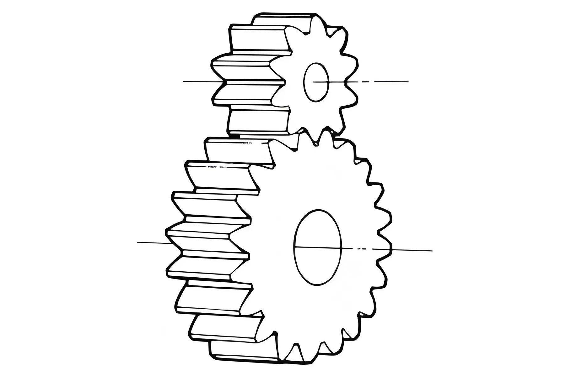
The two-stage spur gear planetary reducer I consider consists of two 2K-H type units connected in series. The sun gear of the first stage serves as the input shaft, connected to a motor. The planet carrier of the first stage acts as the output for that stage and the input for the second stage, linked to the sun gear of the second stage. Finally, the planet carrier of the second stage is the output shaft, connected to the load mechanism. This configuration allows for high reduction ratios in a compact space, making it ideal for applications where size and weight are critical. The use of spur gears in this setup ensures straightforward manufacturing and efficient power transmission.
Determination of Design Variables
In optimizing the spur gear planetary reducer, the primary design parameters include the module (m), number of teeth (z), profile shift coefficient (x), pressure angle (α), and face width (b). However, for this two-stage reducer, given the input power P, speed n, total transmission ratio i₀, and number of planet gears nₚ, the volume largely depends on m, z, b, and x. Since all spur gears share the same module, and the numbers of teeth and profile shift coefficients are interrelated due to meshing conditions and total transmission ratio constraints, I select independent design variables. Specifically, after analyzing the gear train, I define the design variable vector as X = [m, z₁, x₁] = [X₁, X₂, X₃], where z₁ is the number of teeth on the first sun gear, and x₁ is its profile shift coefficient. This simplification reduces complexity while capturing the essential factors affecting volume.
To elaborate, the module m is a discrete variable typically standardized in gear design. The number of teeth z₁ influences the gear ratios and sizes of all other spur gears in the system. The profile shift coefficient x₁ affects the tooth geometry and strength. By optimizing these variables, I aim to achieve a balance between size reduction and performance. Table 1 summarizes the design variables and their roles in the spur gear planetary reducer.
| Variable | Symbol | Description | Type |
|---|---|---|---|
| Module | m | Standardized gear size parameter | Discrete |
| Number of teeth (first sun gear) | z₁ | Determines gear ratios and sizes | Integer |
| Profile shift coefficient (first sun gear) | x₁ | Affects tooth geometry and strength | Continuous |
Establishment of the Objective Function
The objective is to minimize the volume of the spur gear planetary reducer, which directly correlates with material usage, weight, and cost. The volume is calculated based on the gear geometries, considering the spur gears’ outer dimensions. For sun gears and planet gears, I use the addendum circle diameter to compute volume, while for ring gears, I consider the difference between the dedendum and addendum circle diameters. The total volume V is expressed as:
$$ V = \frac{\pi}{4} \left[ b_1 d_{a1}^2 + n_{p1} b_2 d_{a2}^2 + b_3 d_{a3}^2 + n_{p2} b_4 d_{a4}^2 + b_5 (d_{f5}^2 – d_{a5}^2) \right] $$
where:
- \( b_1, b_2, b_3, b_4, b_5 \) are the face widths of gears 1 (first sun), 2 (first planet), 3 (second sun), 4 (second planet), and 5 (ring gear), respectively.
- \( d_{a1}, d_{a2}, d_{a3}, d_{a4}, d_{a5} \) are the addendum circle diameters.
- \( d_{f5} \) is the dedendum circle diameter of the ring gear.
- \( n_{p1} \) and \( n_{p2} \) are the numbers of planet gears in the first and second stages, respectively.
The addendum circle diameter for a spur gear is given by \( d_a = d + 2h_a \), where \( d \) is the pitch diameter and \( h_a \) is the addendum. For standard spur gears, \( h_a = m \cdot h_a^* \), with \( h_a^* \) as the addendum coefficient. The dedendum circle diameter is \( d_f = d – 2h_f \), where \( h_f = m \cdot (h_a^* + c^*) \), and \( c^* \) is the clearance coefficient. The profile shift affects these dimensions, so I incorporate the profile shift coefficients \( x_1, x_2, x_3, x_4, x_5 \) into the calculations. The total volume function thus becomes a complex expression involving m, z, x, and b, which I aim to minimize.
To simplify, I assume all spur gears have the same module m and standard pressure angle α. The face widths are derived from empirical relationships: \( b_1 = k_1 m \), \( b_2 = k_2 m \), etc., where \( k_i \) are constants based on design practice. However, for optimization, I treat face widths as dependent variables, constrained by geometric limits. The objective function is nonlinear and involves both discrete and continuous variables, making it suitable for hybrid optimization techniques.
Formulation of Constraint Conditions
The optimization must satisfy multiple constraints to ensure the spur gear planetary reducer functions correctly and reliably. I categorize these into gear meshing constraints, strength constraints, and other practical constraints. Each category includes specific conditions derived from gear theory and design standards.
Gear Meshing Constraints
These constraints ensure proper assembly and operation of the spur gears in the planetary system.
1. Transmission Ratio Condition: The total transmission ratio \( i_0 \) is fixed based on application requirements. For the two-stage reducer, \( i_0 = i_{1H1} \times i_{3H2} \), where \( i_{1H1} \) is the ratio of the first stage and \( i_{3H2} \) is the ratio of the second stage. For a spur gear planetary system, these ratios depend on the numbers of teeth. Specifically:
$$ i_{1H1} = 1 + \frac{z_5}{z_1}, \quad i_{3H2} = 1 + \frac{z_5}{z_3} $$
where \( z_5 \) is the number of teeth on the ring gear, and \( z_3 \) is the number of teeth on the second sun gear. Since \( i_0 \) is given, this imposes a relation between \( z_1, z_3, \) and \( z_5 \).
2. Concentricity Condition: This ensures that all spur gears mesh properly without interference. For each stage, the center distances between sun-planet and planet-ring pairs must be equal. For the first stage:
$$ \frac{m(z_1 + z_2)}{2 \cos \alpha_{12}} = \frac{m(z_5 – z_2)}{2 \cos \alpha_{25}} $$
where \( \alpha_{12} \) and \( \alpha_{25} \) are the operating pressure angles for the sun-planet and planet-ring meshes, respectively. Similarly, for the second stage:
$$ \frac{m(z_3 + z_4)}{2 \cos \alpha_{34}} = \frac{m(z_5 – z_4)}{2 \cos \alpha_{45}} $$
These equations link the numbers of teeth and profile shift coefficients for spur gears.
3. Adjacency Condition: To prevent planet gears from colliding, the addendum circle diameters of planet gears must be less than twice the center distance multiplied by the sine of the angle between adjacent planets. For the first stage:
$$ d_{a2} < 2 a_{12} \sin \frac{\pi}{n_{p1}} $$
For the second stage:
$$ d_{a4} < 2 a_{34} \sin \frac{\pi}{n_{p2}} $$
where \( a_{12} \) and \( a_{34} \) are the center distances.
4. Assembly Condition: The numbers of teeth must allow even distribution of planet gears. For spur gear planetary systems, this requires:
$$ \frac{z_1 + z_5}{n_{p1}} \in \mathbb{Z}, \quad \frac{z_3 + z_5}{n_{p2}} \in \mathbb{Z} $$
where \( \mathbb{Z} \) denotes integers.
Strength Constraints
Spur gears must withstand operational loads without failure. I focus on contact stress and bending stress constraints for the sun gears, as they are typically critical components.
1. Contact Stress Constraint: The contact stress \( \sigma_H \) must not exceed the allowable stress \( [\sigma_H] \). For spur gears, based on ISO standards:
$$ \sigma_H = Z_H Z_E Z_{\epsilon} Z_{\beta} \sqrt{ \frac{F_t}{d b} \cdot \frac{u \pm 1}{u} } \leq [\sigma_H] $$
where:
- \( Z_H \) is the zone factor.
- \( Z_E \) is the elasticity factor.
- \( Z_{\epsilon} \) is the contact ratio factor.
- \( Z_{\beta} \) is the helix angle factor (equal to 1 for spur gears).
- \( F_t \) is the tangential force.
- \( d \) is the pitch diameter.
- \( b \) is the face width.
- \( u \) is the gear ratio.
For the first sun gear (spur gear 1):
$$ \sigma_{H1} = Z_{H1} Z_{E} Z_{\epsilon 1} \sqrt{ \frac{F_{t1}}{d_1 b_1} \cdot \frac{u_1 + 1}{u_1} } \leq [\sigma_{H1}] $$
Similarly for the second sun gear (spur gear 3). The tangential forces account for load sharing among planet gears.
2. Bending Stress Constraint: The bending stress \( \sigma_F \) must not exceed the allowable stress \( [\sigma_F] \). For spur gears:
$$ \sigma_F = \frac{F_t}{b m} Y_{Fa} Y_{Sa} Y_{\epsilon} Y_{\beta} \leq [\sigma_F] $$
where:
- \( Y_{Fa} \) is the form factor.
- \( Y_{Sa} \) is the stress correction factor.
- \( Y_{\epsilon} \) is the bending contact ratio factor.
- \( Y_{\beta} \) is the helix angle factor (equal to 1 for spur gears).
For the first sun gear:
$$ \sigma_{F1} = \frac{F_{t1}}{b_1 m} Y_{Fa1} Y_{Sa1} Y_{\epsilon 1} \leq [\sigma_{F1}] $$
And similarly for the second sun gear.
Other Constraints
These include practical design limits for spur gears:
- Module Limit: \( m \geq 2 \) mm for power transmission.
- Face Width Limits: Based on gear design practice, \( 5 \leq b/m \leq 17 \) for the first stage and \( 8 \leq b/m \leq 25 \) for the second stage.
- Pressure Angle Limits: For external spur gear meshes, \( \alpha = 24^\circ \text{ to } 30^\circ \); for internal meshes, \( \alpha = 17.5^\circ \text{ to } 23^\circ \).
- Planet Gear Count: Typically, \( n_{p1} = n_{p2} = 3 \) for balance and load distribution.
Table 2 summarizes all constraints for quick reference.
| Category | Constraint | Mathematical Expression |
|---|---|---|
| Gear Meshing | Transmission Ratio | \( i_0 = (1 + z_5/z_1) \times (1 + z_5/z_3) \) |
| Concentricity | \( (z_1 + z_2)/\cos \alpha_{12} = (z_5 – z_2)/\cos \alpha_{25} \) and similarly for second stage | |
| Adjacency | \( d_{a2} < 2 a_{12} \sin(\pi/n_{p1}) \), \( d_{a4} < 2 a_{34} \sin(\pi/n_{p2}) \) | |
| Assembly | \( (z_1 + z_5)/n_{p1} \in \mathbb{Z} \), \( (z_3 + z_5)/n_{p2} \in \mathbb{Z} \) | |
| Strength | Contact Stress | \( \sigma_{H1} \leq [\sigma_{H1}] \), \( \sigma_{H3} \leq [\sigma_{H3}] \) |
| Bending Stress | \( \sigma_{F1} \leq [\sigma_{F1}] \), \( \sigma_{F3} \leq [\sigma_{F3}] \) | |
| Other | Module | \( m \geq 2 \) |
| Face Width | \( 5 \leq b_1/m \leq 17 \), \( 8 \leq b_3/m \leq 25 \) | |
| Pressure Angle | \( 24^\circ \leq \alpha_{12}, \alpha_{34} \leq 30^\circ \), \( 17.5^\circ \leq \alpha_{25}, \alpha_{45} \leq 23^\circ \) | |
| Planet Gear Count | \( n_{p1} = n_{p2} = 3 \) |
Optimization Methodology: Hybrid Discrete Variable Approach
Given the nature of the design variables—module m is discrete, while z₁ is integer and x₁ is continuous—I employ a hybrid discrete variable optimization method. This approach combines discrete and continuous optimization techniques to handle the mixed-variable problem efficiently. The core algorithm is based on the discrete complex method, which iteratively refines a set of points in the design space toward the optimum.
The optimization problem is formulated as:
$$ \min_{X} V(X) \quad \text{subject to} \quad g_j(X) \leq 0, \quad j = 1, 2, \ldots, 17 $$
where X = [m, z₁, x₁], V is the volume objective function, and g_j are the constraint functions derived from the conditions above.
The steps of the hybrid discrete variable optimization method are as follows:
- Discretization: Continuous variables like x₁ are discretized uniformly to transform the problem into a fully discrete domain. For example, x₁ is rounded to increments of 0.01 for practical purposes.
- Initial Discrete Complex Formation: Generate an initial set of k discrete points (vertices) in the design space, where n+1 ≤ k ≤ 2n, with n being the number of design variables (here, n=3). These points must satisfy the variable bounds. For instance, I start with a feasible point X⁽⁰⁾ = [m₀, z₁₀, x₁₀] and then create additional points by perturbing each variable within its discrete steps.
- Evaluation and Sorting: Calculate the objective function V(X) and constraint violations for each vertex. Define an effective objective function Ef(X) that penalizes constraint violations, guiding the search toward feasible regions. For example:
$$ Ef(X) = V(X) + \rho \sum_{j=1}^{17} \max(0, g_j(X))^2 $$
where ρ is a penalty factor. Sort the vertices based on Ef(X), identifying the worst point X⁽ᴴ⁾ and the best point X⁽ᴸ⁾. - Search Direction and Step: Compute the centroid X⁽ᶜ⁾ of the remaining vertices (excluding X⁽ᴴ⁾). Define a search direction S = X⁽ᶜ⁾ – X⁽ᴴ⁾. Perform a one-dimensional discrete search along S with a step length factor α to find a new point X⁽ᵀ⁾. The step length is adjusted based on success or failure in improving Ef(X).
- Iteration and Refinement: If X⁽ᵀ⁾ is better than X⁽ᴴ⁾, replace X⁽ᴴ⁾ with X⁽ᵀ⁾ and increase α to accelerate convergence. Otherwise, decrease α and repeat the search. If α falls below a minimum threshold without improvement, use restart techniques or auxiliary functions like reflection to explore new regions.
- Convergence Check: The algorithm terminates when the discrete complex vertices converge, i.e., the maximum distance between vertices in any variable direction is less than the discrete increment for that variable. Additionally, the number of variables with changes below their increments should be below a preset limit (e.g., 1 to n).
- Final Refinement: After convergence, perform a local search in the neighborhood of the best point to ensure no better solutions are missed. This includes checking adjacent discrete values for m and z₁, and small perturbations for x₁.
This method efficiently handles the mixed discrete-continuous nature of spur gear design parameters. The discrete complex ensures exploration of the feasible space, while the one-dimensional search and penalty functions drive the solution toward optimality. Table 3 outlines the algorithm parameters used in the optimization.
| Parameter | Symbol | Value/Range | Description |
|---|---|---|---|
| Number of vertices | k | 6 to 8 | Based on n=3 design variables |
| Penalty factor | ρ | 1000 | For constraint violation penalty |
| Step length factor initial | α₀ | 1.0 | Initial step multiplier |
| Minimum step length factor | α_min | 0.01 | Threshold for step reduction |
| Discrete increments | Δm, Δz₁, Δx₁ | 0.5 mm, 1, 0.01 | Steps for module, teeth, and shift coefficient |
To illustrate the optimization process, consider a numerical example. Suppose the input requirements are: power P = 10 kW, input speed n = 1500 rpm, total transmission ratio i₀ = 30, and planet gear count nₚ = 3 per stage. Using the hybrid discrete variable method, I iteratively adjust m, z₁, and x₁. For instance, starting with m = 2 mm, z₁ = 20, x₁ = 0, the algorithm evaluates constraints and volume, then moves toward better points. After convergence, the optimal solution might be m = 2.5 mm, z₁ = 18, x₁ = 0.2, resulting in a volume reduction of 15% compared to initial design. The spur gears in this configuration meet all strength and meshing requirements while minimizing material usage.
Discussion on Spur Gear Design Implications
The optimization of spur gear planetary reducers highlights several key insights. First, the module m has a significant impact on volume; larger modules increase gear size but may allow fewer teeth for the same ratio, so a balance is essential. Second, the profile shift coefficient x₁ is crucial for adjusting tooth geometry to meet strength constraints without increasing volume. In spur gears, positive profile shift can enhance bending strength by thickening the tooth root, while negative shift might reduce interference in internal meshes. Third, the number of teeth z₁ affects not only the transmission ratio but also the gear diameters and thus the overall volume. By optimizing these variables simultaneously, I achieve a compact design that leverages the advantages of spur gears: simplicity, low cost, and high efficiency.
Furthermore, the hybrid discrete variable method proves effective for such problems because it accommodates the real-world discreteness of gear parameters. Standard modules are discrete, and tooth counts are integers, so continuous optimization methods might yield impractical solutions requiring rounding. This method directly searches the discrete space, ensuring feasible and manufacturable designs. Additionally, the use of spur gears simplifies the constraint formulations, as their geometry is well-defined and standardized.
In practice, the optimized spur gear planetary reducer can be applied in various industries. For example, in automotive transmissions, reducing volume and weight contributes to fuel efficiency. In robotics, compact reducers enable more agile and lightweight manipulators. The optimization framework I present is flexible and can be adapted to different specifications by modifying the constraints or objective function, such as minimizing noise or maximizing efficiency.
Conclusion
In this article, I have detailed the optimization design of a two-stage spur gear planetary reducer, focusing on volume minimization through a hybrid discrete variable approach. The design variables—module, number of teeth, and profile shift coefficient—are carefully selected to capture the essence of the problem. The objective function and constraints are derived from gear theory, ensuring functional and reliable performance. The optimization method efficiently handles mixed discrete-continuous variables, converging to practical solutions. This approach demonstrates significant benefits over traditional design, including material savings, cost reduction, and improved performance. As spur gears continue to be vital in mechanical systems, such optimization techniques provide valuable tools for engineers seeking to enhance design efficiency and effectiveness.
Future work could explore multi-objective optimization, considering factors like thermal performance or dynamic behavior. Additionally, integrating advanced materials or manufacturing constraints could further refine the design. Nonetheless, the current methodology offers a robust foundation for optimizing spur gear planetary reducers, contributing to the advancement of compact and high-performance mechanical transmissions.