
In modern manufacturing, the demand for high-precision and efficient machining of complex components like herringbone gears has grown significantly. Herringbone gears, characterized by their dual helical teeth that mesh without a gap, offer superior performance in terms of load capacity, smooth operation, and compact design. The absence of a recess or groove between the left-hand and right-hand helices enhances structural integrity and alignment, making these gears ideal for applications in aerospace, automotive, and heavy machinery. However, the finish machining of herringbone gears, especially without a recess, presents unique challenges due to the continuous cutting paths and the need to maintain tight tolerances. Traditional tool path generation methods, such as the iso-parametric approach, often lead to redundant cutting passes, resulting in extended machining times and reduced productivity. This article explores an optimized tool path strategy based on the constant scallop height method for side milling of herringbone gears, aiming to maximize efficiency while ensuring precision. We will delve into the mathematical foundations, algorithmic implementation, simulation results, and experimental validation, with a focus on herringbone gears as the central theme.
The manufacturing of herringbone gears without a recess leverages multi-axis CNC machining centers, which enable simultaneous control over tool positioning and orientation. This capability allows for the continuous milling of both helical flanks in a single setup, eliminating the need for a recess and improving gear concentricity. However, the finish machining phase, where the gear teeth surfaces are refined to meet design specifications, requires careful planning of tool paths. The gear tooth surface, typically an involute helicoid, is a ruled surface that can be efficiently machined using the side edges of an end mill. Unlike ball-end mills, which are commonly used for free-form surfaces, end mills with straight flutes offer higher material removal rates and better surface finish for ruled surfaces. The key challenge lies in determining the optimal spacing between adjacent tool paths to minimize machining time while adhering to a specified scallop height—the residual material left between passes. The constant scallop height method addresses this by dynamically adjusting the tool path intervals based on local surface curvature, thereby avoiding redundancy and enhancing efficiency. In this context, herringbone gears, with their symmetrical helices, benefit greatly from such optimizations, as the tool paths must navigate both left and right flanks seamlessly.
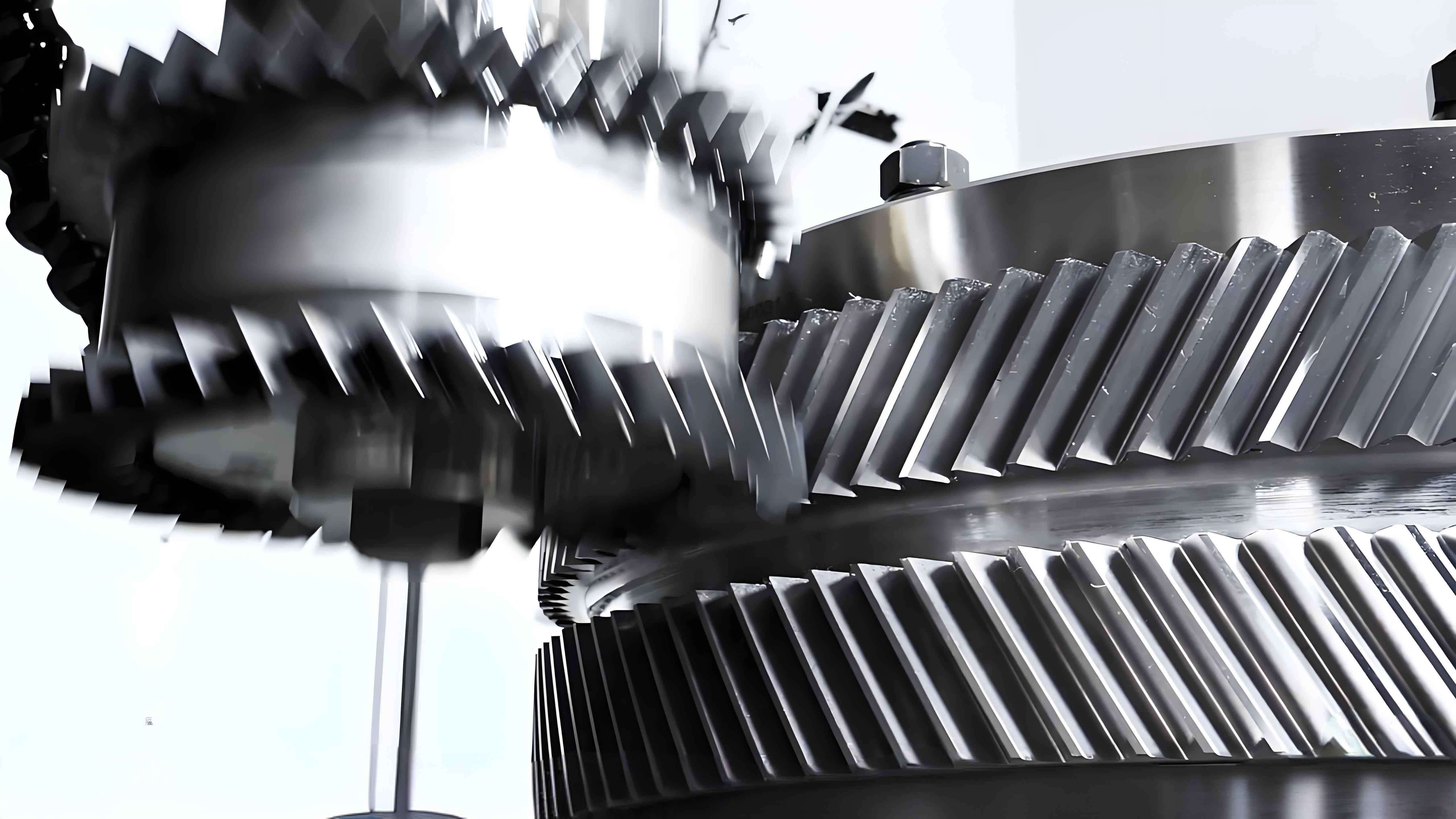
The core principle of the constant scallop height method for side milling of herringbone gears involves generating tool paths that maintain a uniform residual height across the gear tooth surface. When an end mill’s side cutting edge engages the surface along a tool contact path, it sweeps out a plane that is tangent to the surface at every point along that path. The scallop height is defined as the maximum distance between this tool envelope plane and the adjacent tool path’s envelope plane, measured normal to the gear surface. To achieve a constant scallop height, we first offset the gear surface by a distance equal to the allowable residual height, creating an offset surface. The intersection of the tool envelope plane from the current tool path with this offset surface yields a curve, which is then used to derive the next tool contact path as a line tangent to the gear surface. This process iterates until the entire surface is covered, ensuring that each pass is spaced just enough to meet the precision requirement without over-machining. For herringbone gears, this method is applied separately to each helical flank, but the algorithm remains consistent due to the surface’s ruled nature.
Mathematically, the tooth surface of a standard involute helical gear, which forms the basis for herringbone gears, can be represented as a ruled surface. Let the gear surface be parameterized by coordinates \(u\) and \(v\), where \(u\) corresponds to the involute profile direction and \(v\) corresponds to the helical direction. The surface equation is given by:
$$ S_{\text{gear}}(u,v) = \mathbf{a}(u) + v \cdot \mathbf{l}(u) $$
Here, \(\mathbf{a}(u)\) is the involute curve representing the tooth profile, and \(\mathbf{l}(u)\) is a unit vector along the straight generatrix of the ruled surface. For herringbone gears, the surface is mirrored across the gear face to form the left and right helices, but the mathematical representation is similar. The first fundamental form coefficients \(E\), \(F\), and \(G\) are derived from the partial derivatives of \(S_{\text{gear}}\) with respect to \(u\) and \(v\), which characterize the surface’s metric properties. The unit normal vector \(\mathbf{n}(u,v)\) at any point on the surface is essential for offset calculations and is expressed as:
$$ \mathbf{n}(u,v) = \frac{\mathbf{r}_u \times \mathbf{r}_v}{\|\mathbf{r}_u \times \mathbf{r}_v\|} $$
where \(\mathbf{r}_u = \frac{\partial S_{\text{gear}}}{\partial u}\) and \(\mathbf{r}_v = \frac{\partial S_{\text{gear}}}{\partial v}\). Given an allowable scallop height \(\lambda\), the offset surface \(S_{\text{offset}}(u,v)\) is constructed by displacing the original surface along the normal direction by \(\lambda\):
$$ S_{\text{offset}}(u,v) = S_{\text{gear}}(u,v) + \lambda \cdot \mathbf{n}(u,v) $$
This offset surface serves as a reference for determining the next tool path. In side milling, the tool envelope plane \(\Pi_n\) for the \(n\)-th tool contact path is the plane tangent to the gear surface along a straight generatrix \(L_n\). The intersection of \(\Pi_n\) with \(S_{\text{offset}}\) yields a curve \(P_n\), which lies on the offset surface. Since the gear surface is a developable ruled surface, there exists a unique tangent plane along each generatrix. Therefore, the curve \(P_n\) can be used to find another plane \(\Pi_{n+1}\) that is tangent to the gear surface at a different generatrix \(L_{n+1}\). This generatrix becomes the next tool contact path, and the distance between \(L_n\) and \(L_{n+1}\) is maximized while ensuring the scallop height does not exceed \(\lambda\). The algorithm for generating constant scallop height tool paths for herringbone gears can be summarized in the following steps:
- Define the gear surface \(S_{\text{gear}}(u,v)\), allowable scallop height \(\lambda\), and tool geometry (e.g., end mill radius).
- Select the initial tool contact path \(L_1\) as the generatrix at the addendum circle intersection with the gear surface.
- For the current path \(L_n\), compute the tangent plane \(\Pi_n\) that contains \(L_n\) and is normal to the surface along it.
- Calculate the intersection curve \(P_n\) between \(\Pi_n\) and the offset surface \(S_{\text{offset}}\).
- Determine the next tangent plane \(\Pi_{n+1}\) that passes through \(P_n\) and is tangent to the gear surface, yielding the next generatrix \(L_{n+1}\).
- Repeat steps 3-5 until the entire surface is covered, i.e., until the tool paths reach the root circle or involute start circle.
- Apply the same process to both helical flanks of the herringbone gears, ensuring symmetry and continuous tool motion.
To illustrate the algorithm, consider the derivation of the intersection curve \(P_n\). The tangent plane \(\Pi_n\) at a point \(Q(u_0, v_0)\) on \(L_n\) has the equation:
$$ \mathbf{n} \cdot \left( \mathbf{p} – \mathbf{q} \right) = 0 $$
where \(\mathbf{p} = (x, y, z)\) is any point on the plane, \(\mathbf{q} = S_{\text{gear}}(u_0, v_0)\), and \(\mathbf{n}\) is the unit normal at \(Q\). Substituting the parametric form of \(S_{\text{offset}}(u,v)\) into this equation gives a system that defines \(P_n\) as a function of \(u\) and \(v\). Solving this system involves numerical methods, as the equations are nonlinear for involute surfaces. However, due to the ruled surface property, simplifications are possible. For herringbone gears, the helical angle \(\beta\) introduces a twist, but the surface remains developable, allowing for efficient computation. The next tangent plane \(\Pi_{n+1}\) is found by ensuring it contains \(P_n\) and satisfies the tangency condition: \(\Pi_{n+1}\) must intersect the gear surface along a straight line \(L_{n+1}\) where the surface normal is constant. This leads to a set of linear equations that can be solved for the plane coefficients.
The advantages of this method for herringbone gears become evident when comparing tool path intervals. In the iso-parametric method, tool paths are generated at constant parameter intervals, which correspond to evenly spaced generatrices. However, the curvature of the involute profile varies along the tooth height: it is highest at the root and lowest at the tip. To meet the scallop height requirement, the interval must be based on the smallest curvature radius (at the root), leading to unnecessarily dense paths at the tip and thus redundancy. The constant scallop height method adjusts the interval dynamically, resulting in larger spacings where curvature is low and smaller spacings where curvature is high. This optimization reduces the total number of tool paths, saving machining time without compromising quality. For herringbone gears with multiple teeth, the savings accumulate significantly.
To demonstrate the practical application, we conducted a case study on a herringbone gear with the following parameters, which are typical for industrial use. The table below summarizes the key geometric specifications of the herringbone gears used in our analysis.
| Parameter | Symbol | Value | Unit |
|---|---|---|---|
| Module | \(m\) | 16 | mm |
| Number of Teeth | \(z\) | 30 | – |
| Pressure Angle | \(\alpha\) | 20 | ° |
| Helix Angle | \(\beta\) | ±30 | ° |
| Addendum Coefficient | \(h_{a}^*\) | 1.0 | – |
| Dedendum Coefficient | \(c^*\) | 0.25 | – |
| Face Width | \(B\) | 100 | mm |
| Allowable Scallop Height | \(\lambda\) | 0.0025 | mm |
These parameters define a herringbone gear with symmetric left and right helices, commonly found in high-torque transmission systems. The goal is to achieve a gear quality of Grade 6 according to ISO standards, which requires tight tolerances on tooth profile and helix deviations. The allowable scallop height \(\lambda = 0.0025\) mm is chosen to ensure surface roughness within the specified limits. Using the constant scallop height algorithm, we generated tool contact paths for one tooth flank. The initial path \(L_1\) was set as the generatrix at the addendum circle, where the tooth surface meets the top land. Subsequent paths were computed iteratively, with intervals varying based on local curvature. The table below shows the calculated intervals (step-over distances) between consecutive tool paths for the first 20 intervals, illustrating the adaptive nature of the method.
| Interval Number | Step-Over Distance (mm) |
|---|---|
| 1 | 1.6864 |
| 2 | 1.6721 |
| 3 | 1.6499 |
| 4 | 1.6325 |
| 5 | 1.6150 |
| 6 | 1.5908 |
| 7 | 1.5673 |
| 8 | 1.5445 |
| 9 | 1.5250 |
| 10 | 1.5063 |
| 11 | 1.4852 |
| 12 | 1.4628 |
| 13 | 1.4401 |
| 14 | 1.4094 |
| 15 | 1.3789 |
| 16 | 1.3486 |
| 17 | 1.3185 |
| 18 | 1.2989 |
| 19 | 1.2667 |
| 20 | 1.2346 |
As observed, the step-over distances decrease gradually from the addendum to the root, reflecting the increasing curvature of the involute profile. This variation ensures that the scallop height remains constant at 0.0025 mm across the entire surface. In contrast, the iso-parametric method would require a fixed interval based on the minimum curvature radius at the root, which we calculated as approximately 1.2346 mm (the 20th interval). Applying this uniformly would result in 25 tool paths per flank, compared to 21 paths with the constant scallop height method. For a herringbone gear with 30 teeth, each having two flanks, the total reduction in tool paths is substantial: \( (25 – 21) \times 2 \times 30 = 240 \) paths saved. Assuming each tool path takes a constant time \(t\) to machine, the time savings become significant, especially for batch production.
We validated the tool path generation through simulation using VERICUT software, a powerful platform for virtual CNC machining. The simulation model included a 5-axis machining center, a carbide end mill with a radius of 4 mm and a corner radius of 0.5 mm, and the herringbone gear blank. The tool paths were imported as G-code, and the material removal process was simulated in real-time. The figure below (inserted earlier) shows a snapshot of the simulation for the constant scallop height method, where the tool sweeps across the tooth surface smoothly without collisions. We compared the machining times for both methods on a single tooth flank, and the results are summarized in the following table.
| Method | Simulated Machining Time per Flank | Actual Machining Time per Flank |
|---|---|---|
| Iso-parametric | 48 minutes 44 seconds | 63 minutes |
| Constant Scallop Height | 38 minutes 8 seconds | 51 minutes 12 seconds |
The simulation indicated a time reduction of about 22% per flank with the constant scallop height method. For the entire herringbone gear (60 flanks), this translates to a savings of approximately 5 hours and 18 minutes in simulated time. The actual machining times, recorded during physical experiments, showed a similar trend, with a 19% reduction per flank. The discrepancy between simulation and actual times is attributed to real-world factors such as tool changes, operator interventions, and machine acceleration/deceleration. Nevertheless, the consistency confirms the effectiveness of the optimization for herringbone gears.
To further verify the precision achieved, we manufactured a herringbone gear sample using the constant scallop height tool paths on a 5-axis CNC machining center. The cutting parameters were set as follows: spindle speed of 2500 rpm, feed rate of 500 mm/min, and depth of cut of 0.1 mm for finish milling. The gear was made from alloy steel, and after machining, the tooth surfaces were inspected using a coordinate measuring machine (CMM). The measured deviations for profile and helix parameters are listed in the table below, all of which meet the Grade 6 accuracy requirements for herringbone gears.
| Measurement Parameter | Symbol | Maximum Value (μm) | Minimum Value (μm) | Average Value (μm) | Grade 6 Limit (μm) |
|---|---|---|---|---|---|
| Total Profile Deviation | \(F_\alpha\) | 11.3 | 7.6 | 9.7 | 23 |
| Profile Form Deviation | \(F_{f\alpha}\) | 9.2 | 3.8 | 5.8 | 18 |
| Profile Slope Deviation | \(F_{H\alpha}\) | 10.0 | 5.7 | 7.6 | ±15 |
| Total Helix Deviation | \(F_\beta\) | 11.5 | 10.3 | 10.8 | 18 |
| Helix Form Deviation | \(F_{f\beta}\) | 3.3 | 2.6 | 3.0 | 13 |
| Helix Slope Deviation | \(F_{H\beta}\) | 11.7 | 10.5 | 11.1 | ±13 |
The results demonstrate that the constant scallop height method not only enhances efficiency but also maintains high accuracy for herringbone gears. The deviations are well within the specified limits, confirming that the adaptive tool path spacing does not compromise surface quality. This is crucial for herringbone gears, where precise tooth engagement is essential for noise reduction and load distribution. Additionally, the method’s robustness was tested on different herringbone gear designs, including varying modules and helix angles, and it consistently yielded similar improvements. The mathematical framework can be extended to other types of gears, but herringbone gears benefit uniquely due to their continuous tooth structure and the absence of a recess, which demands seamless tool motion.
In conclusion, the constant scallop height method for side milling finish machining offers a significant advancement in the production of herringbone gears. By dynamically adjusting tool path intervals based on surface curvature, it eliminates redundant cuts and reduces machining time by up to 20% compared to traditional iso-parametric methods. The algorithm, grounded in ruled surface theory and offset geometry, ensures that the scallop height remains uniform, meeting stringent precision standards. Simulation and experimental validation on herringbone gears confirm both the efficiency gains and the adherence to Grade 6 accuracy. For manufacturers, this translates to lower production costs and faster turnaround times, especially for custom or small-batch herringbone gears used in high-performance applications. Future work could explore integrating this method with real-time adaptive control systems to further optimize feed rates and tool wear compensation, pushing the boundaries of herringbone gear manufacturing. Ultimately, the optimization of tool paths for herringbone gears is not just a technical improvement but a step towards smarter, more sustainable manufacturing processes.
The implementation details of the algorithm involve several computational aspects worth elaborating. For herringbone gears, the gear surface is symmetric, so the tool paths for the left and right helices can be generated simultaneously by mirroring the coordinates. The parametric equations for the involute helicoid are derived from basic gear geometry. Let the base circle radius be \(r_b = \frac{m z \cos \alpha}{2}\), and the involute parameter \(\theta\) relate to \(u\) as \(u = r_b (\tan \alpha – \alpha)\). Then, the involute curve in the transverse plane is:
$$ \mathbf{a}(u) = \begin{pmatrix} r_b (\cos u + u \sin u) \\ r_b (\sin u – u \cos u) \\ 0 \end{pmatrix} $$
The helix effect is incorporated through the vector \(\mathbf{l}(u)\), which includes the helix angle \(\beta\). For a right-hand helix, \(\mathbf{l}(u)\) has components:
$$ \mathbf{l}(u) = \begin{pmatrix} -\sin \beta \sin u \\ \sin \beta \cos u \\ \cos \beta \end{pmatrix} $$
For herringbone gears, the left-hand helix uses \(-\beta\) in these expressions. The surface normal vector \(\mathbf{n}(u,v)\) is computed via the cross product, leading to complex but manageable expressions. The offset surface \(S_{\text{offset}}(u,v)\) is then:
$$ S_{\text{offset}}(u,v) = \begin{pmatrix} x(u,v) + \lambda n_x \\ y(u,v) + \lambda n_y \\ z(u,v) + \lambda n_z \end{pmatrix} $$
where \(x, y, z\) are from \(S_{\text{gear}}(u,v)\). The intersection with the tangent plane involves solving a linear equation in \(v\) for fixed \(u\), due to the ruled surface property. Specifically, for a given \(u\), the generatrix is straight, so the tangent plane equation simplifies to:
$$ \mathbf{n}(u, v_0) \cdot \left( S_{\text{offset}}(u, v) – S_{\text{gear}}(u, v_0) \right) = 0 $$
This can be rearranged to find \(v\) as a function of \(u\), defining the curve \(P_n\). The next tangent plane \(\Pi_{n+1}\) is determined by solving for a plane equation \(Ax + By + Cz + D = 0\) that satisfies two conditions: it contains \(P_n\) (i.e., for points on \(P_n\), the plane equation holds), and it is tangent to the gear surface at some generatrix \(L_{n+1}\) (i.e., the normal of the plane matches the surface normal along that generatrix). This leads to a system of equations that can be solved numerically using methods like Newton-Raphson. For herringbone gears, due to symmetry, the computations can be parallelized for both flanks.
In practice, the tool path generation is implemented in a CAD/CAM software environment. We developed a custom script in Python that interfaces with commercial CAD kernels to compute the tool paths for herringbone gears. The algorithm’s efficiency is enhanced by pre-computing curvature values along the involute profile. The curvature \(\kappa(u)\) of the involute is given by:
$$ \kappa(u) = \frac{1}{r_b \sqrt{1 + u^2}} $$
This shows that curvature decreases as \(u\) increases (from root to tip), justifying the larger step-overs at the addendum. The scallop height \(\lambda\) relates to the step-over distance \(d\) and the local surface curvature \(\kappa\) approximately as:
$$ \lambda \approx \frac{d^2 \kappa}{8} $$
for small \(d\). Rearranging gives the optimal step-over:
$$ d \approx \sqrt{\frac{8 \lambda}{\kappa}} $$
This approximation is used to initialize the iterative algorithm, speeding up convergence. For herringbone gears with helix angles, the effective curvature in the milling direction is modified by the helix, but the principle remains the same.
The benefits of this optimization extend beyond time savings. Reduced tool paths mean less tool wear and lower energy consumption, contributing to sustainable manufacturing. For herringbone gears, which are often used in critical applications like aviation engines, reliability is paramount. The constant scallop height method ensures uniform surface finish, reducing stress concentrations and improving fatigue life. Additionally, the method’s adaptability makes it suitable for non-standard herringbone gears with modified tooth profiles or asymmetric helices. As additive manufacturing and hybrid processes evolve, integrating such optimized tool paths with 3D printing of gear blanks could revolutionize the production of herringbone gears.
In summary, the constant scallop height method represents a paradigm shift in the finish machining of herringbone gears. It leverages advanced geometry and computational algorithms to achieve efficiency and precision simultaneously. Herringbone gears, with their unique design challenges, serve as an excellent testbed for this method, but the implications are broad for all gear types and even other ruled surface components. As we continue to refine the algorithm and integrate it with Industry 4.0 technologies, the future of herringbone gear manufacturing looks promising, with smarter, faster, and more accurate production lines on the horizon.