
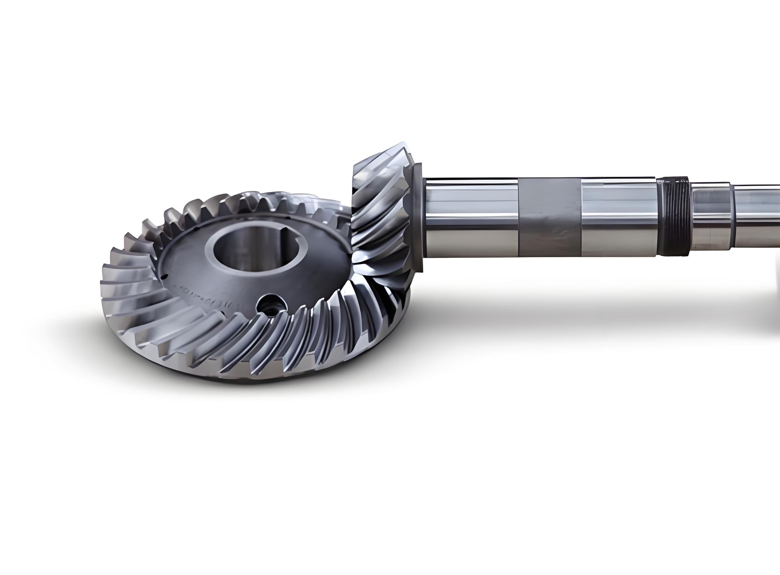
Spiral bevel gears are critical components in power transmission systems, renowned for their high efficiency, smooth operation, significant load-bearing capacity, and low noise and vibration. These attributes make them indispensable in demanding sectors such as automotive, aerospace, and heavy machinery. The pursuit of manufacturing excellence, driven by goals of green production and technological innovation, places stringent demands on the precision, quality, and surface integrity of these gears. A key aspect of surface integrity arising from the machining process is the induction of residual stresses. These stresses, locked within the material after cutting, significantly influence the gear’s dimensional accuracy, fatigue life, wear resistance, and overall reliability. Therefore, a profound understanding of the mechanisms governing residual stress formation during the cutting of spiral bevel gears is paramount. This knowledge is essential for optimizing machining processes, ultimately enhancing product quality and extending service life. This study focuses on investigating the influence of cutting parameters on residual stresses in spiral bevel gears, employing finite element simulation and advanced statistical analysis to derive an optimal parameter set.
1. Machining Methodology and Finite Element Modeling
The tooth cutting of spiral bevel gears is based on the principle of an imaginary crown gear. In this process, a hypothetical generating gear, concentric with the machine cradle, meshes with the gear blank. The cutting edges of the tool represent the teeth of this imaginary gear, progressively generating the tooth profile on the blank. Among various methods, form cutting is employed here, where the tool profile corresponds to the gear tooth space. The cutting process for spiral bevel gears is inherently complex and cannot be simplified as a two-dimensional orthogonal cut. To make the finite element analysis (FEA) computationally feasible while retaining physical fidelity, a localized micro-segment of the cutting process is analyzed. This approach leads to the establishment of an equivalent three-dimensional oblique cutting model, which accurately captures the essential mechanics, including the tool’s inclination angle (λs).
1.1 Workpiece Material and Constitutive Model
The workpiece material is AISI 4340 steel (equivalent to 40CrNiMoA), a high-strength alloy steel commonly used for critical components like gears and shafts due to its excellent strength, toughness, and fatigue resistance. Its physical properties are listed in Table 1.
| Property | Value |
|---|---|
| Density (T/mm³) | 7.83 × 10⁻⁹ |
| Elastic Modulus (MPa) | 2.0 × 10⁵ |
| Poisson’s Ratio | 0.29 |
| Yield Strength (MPa) | 792 |
| Tensile Strength (MPa) | 980 |
The cutting process involves severe plastic deformation, high strain rates, and significant thermal effects. The Johnson-Cook (J-C) constitutive model is employed to capture these coupled phenomena, as it effectively models strain hardening, strain rate sensitivity, and thermal softening. The flow stress is given by:
$$ \sigma = \left[ A + B\left(\varepsilon_{pl}\right)^n \right] \left[ 1 + C \ln\left(\frac{\dot{\varepsilon}_{pl}}{\dot{\varepsilon}_0}\right) \right] \left[ 1 – \left( \frac{T – T_0}{T_m – T_0} \right)^m \right] $$
where $\sigma$ is the equivalent flow stress, $\varepsilon_{pl}$ is the equivalent plastic strain, $\dot{\varepsilon}_{pl}$ is the plastic strain rate, $\dot{\varepsilon}_0$ is the reference strain rate, $T$ is the current temperature, $T_0$ is the room temperature, and $T_m$ is the melting temperature. The parameters $A$, $B$, $C$, $n$, and $m$ are material constants, listed in Table 2 for AISI 4340 steel.
| A (MPa) | B (MPa) | C | n | m |
|---|---|---|---|---|
| 792 | 510 | 0.014 | 0.26 | 1.03 |
1.2 Chip Separation and Friction Modeling
Material separation and chip formation are governed by the Johnson-Cook damage initiation criterion. Damage is assumed to occur when the damage parameter $\omega$ exceeds 1:
$$ \omega = \sum \frac{\Delta \varepsilon_{pl}}{\varepsilon_{pl}^f} $$
The failure strain $\varepsilon_{pl}^f$ is defined as:
$$ \varepsilon_{pl}^f = \left[ D_1 + D_2 \exp\left(D_3 \frac{p}{q}\right) \right] \left[ 1 + D_4 \ln\left(\frac{\dot{\varepsilon}_{pl}}{\dot{\varepsilon}_0}\right) \right] \left[ 1 + D_5 \left( \frac{T – T_0}{T_m – T_0} \right) \right] $$
where $D_1$ to $D_5$ are failure parameters, $p$ is the hydrostatic pressure, and $q$ is the Mises equivalent stress. The failure parameters for AISI 4340 steel are listed in Table 3.
| D₁ | D₂ | D₃ | D₄ | D₅ |
|---|---|---|---|---|
| 0.05 | 3.44 | -2.12 | 0.002 | 0.61 |
The interaction at the tool-chip interface is modeled using a modified Coulomb friction law, which accounts for both sticking and sliding regions:
$$ \tau_c = \begin{cases} \mu \sigma_n & \text{for } \mu \sigma_n < \tau_s \quad \text{(Sliding Region)} \\ \tau_s & \text{for } \mu \sigma_n \ge \tau_s \quad \text{(Sticking Region)} \end{cases} $$
where $\tau_c$ is the frictional shear stress, $\sigma_n$ is the normal stress at the interface, $\tau_s$ is the shear yield strength of the workpiece material, and $\mu$ is the friction coefficient, set to 0.3 in this study.
1.3 Simulation Procedure and Residual Stress Extraction
The simulation of residual stress development is conducted in four sequential stages: (1) the cutting stage, where the tool engages the workpiece; (2) the unloading stage, where tool forces and constraints are removed; (3) the constraint conversion stage, where new boundary conditions are applied to prevent rigid body motion; and (4) the cooling stage, where the workpiece temperature is brought back to room temperature to isolate mechanically induced residual stresses from thermal effects. After simulation completion, the residual stress component in the cutting direction (S11) is extracted. A sampling path is defined beneath the machined surface, avoiding edge effects. Sixty data points are averaged at each depth layer to obtain a representative through-thickness residual stress profile for analysis.
2. Experimental Design and Simulation Results
2.1 Single-Factor Analysis of Residual Stress Distribution
Initial single-factor simulations were conducted to understand the fundamental distribution of residual stresses after cutting spiral bevel gears. With feed rate and depth of cut held constant, the cutting speed was varied. The resulting subsurface residual stress profiles are shown in Figure 1 (conceptual). A consistent trend is observed: the machined surface exhibits tensile residual stress. As depth increases, this tensile stress decreases, transitions into compressive stress, reaches a maximum compressive value, and finally attenuates to zero. This profile is characteristic of machined surfaces and arises from the interplay of mechanical deformation (ploughing, plastic flow) and thermal effects. Higher cutting speeds generate more heat, increasing surface tensile stress due to thermal expansion and subsequent constraint during cooling, while simultaneously softening the material and reducing the subsurface compressive stress induced by mechanical deformation.
2.2 Orthogonal Experiment Design and Results
To systematically investigate the influence and interaction of cutting parameters, an orthogonal experiment array L₂₅(5³) was designed. The factors and their levels are detailed in Table 4.
| Level | Cutting Speed, v (m/min) | Feed Rate, f (mm/rev) | Depth of Cut, ap (mm) |
|---|---|---|---|
| 1 | 75 | 0.1 | 1.0 |
| 2 | 115 | 0.2 | 1.5 |
| 3 | 155 | 0.3 | 2.0 |
| 4 | 195 | 0.4 | 2.5 |
| 5 | 235 | 0.5 | 3.0 |
The simulation results for the 25 trials, reporting the maximum surface tensile residual stress (S₁) and the maximum subsurface compressive residual stress (S₂), are presented in Table 5.
| Trial | v (m/min) | f (mm/rev) | ap (mm) | S₁ (MPa) | S₂ (MPa) |
|---|---|---|---|---|---|
| 1 | 75 | 0.1 | 1.0 | 217.68 | -307.88 |
| 2 | 75 | 0.2 | 1.5 | 245.32 | -329.84 |
| 3 | 75 | 0.3 | 2.0 | 275.38 | -362.70 |
| 4 | 75 | 0.4 | 2.5 | 310.24 | -392.52 |
| 5 | 75 | 0.5 | 3.0 | 347.12 | -428.41 |
| 6 | 115 | 0.1 | 1.5 | 246.51 | -282.36 |
| 7 | 115 | 0.2 | 2.0 | 273.43 | -301.25 |
| 8 | 115 | 0.3 | 2.5 | 304.78 | -341.71 |
| 9 | 115 | 0.4 | 3.0 | 334.11 | -369.28 |
| 10 | 115 | 0.5 | 1.0 | 358.24 | -408.13 |
| 11 | 155 | 0.1 | 2.0 | 263.56 | -235.28 |
| 12 | 155 | 0.2 | 2.5 | 295.83 | -275.15 |
| 13 | 155 | 0.3 | 3.0 | 331.21 | -309.16 |
| 14 | 155 | 0.4 | 1.0 | 354.95 | -338.24 |
| 15 | 155 | 0.5 | 1.5 | 389.45 | -375.77 |
| 16 | 195 | 0.1 | 2.5 | 292.94 | -216.25 |
| 17 | 195 | 0.2 | 3.0 | 319.39 | -238.14 |
| 18 | 195 | 0.3 | 1.0 | 336.79 | -273.44 |
| 19 | 195 | 0.4 | 1.5 | 373.42 | -305.74 |
| 20 | 195 | 0.5 | 2.0 | 412.27 | -334.46 |
| 21 | 235 | 0.1 | 3.0 | 322.50 | -191.15 |
| 22 | 235 | 0.2 | 1.0 | 338.19 | -210.85 |
| 23 | 235 | 0.3 | 1.5 | 371.44 | -242.75 |
| 24 | 235 | 0.4 | 2.0 | 408.24 | -274.65 |
| 25 | 235 | 0.5 | 2.5 | 443.75 | -322.15 |
3. Grey Relational Analysis for Multi-Objective Optimization
To optimize the multiple and often conflicting responses—minimizing surface tensile stress (S₁) and maximizing subsurface compressive stress (S₂)—a Grey Relational Analysis (GRA) was performed. GRA converts a multi-response problem into a single-response optimization using grey relational grade (GRG).
3.1 Data Pre-processing
The experimental data (S₁, S₂) were normalized to make them dimensionless and comparable. Since S₁ is a “lower-the-better” (cost-type) characteristic and S₂ is a “higher-the-better” (benefit-type) characteristic, they were normalized using Eqs. (1) and (2), respectively:
$$ y_i(k) = \frac{\max x_i^0(k) – x_i^0(k)}{\max x_i^0(k) – \min x_i^0(k)} \quad \text{(for S₁)} $$
$$ y_i'(k) = \frac{x_i^0(k) – \min x_i^0(k)}{\max x_i^0(k) – \min x_i^0(k)} \quad \text{(for S₂)} $$
where $x_i^0(k)$ is the original sequence for the k-th response in the i-th experiment.
3.2 Calculation of Grey Relational Coefficient and Grade
The grey relational coefficient $\gamma_i(k)$ was calculated to express the relationship between the ideal (best) and actual normalized experimental results:
$$ \gamma_i(k) = \frac{\Delta_{min} + \xi \Delta_{max}}{\Delta_{0i}(k) + \xi \Delta_{max}} $$
where $\Delta_{0i}(k) = |1 – y_i(k)|$ is the deviation sequence, $\Delta_{min}$ and $\Delta_{max}$ are the minimum and maximum values of $\Delta_{0i}(k)$ for all responses, and $\xi$ is the distinguishing coefficient, set to 0.5. The overall Grey Relational Grade (GRG) $G_i$ for the i-th experiment is the average of the relational coefficients:
$$ G_i = \frac{1}{m} \sum_{k=1}^{m} \gamma_i(k) $$
where $m=2$ is the number of responses. A higher GRG indicates that the corresponding parameter combination is closer to the ideal optimal performance. The processed data and calculated GRG values are shown in Table 6.
| Trial | Normalized S₁ (yᵢ) | Normalized S₂ (yᵢ’) | GRC for S₁ | GRC for S₂ | Grey Relational Grade (Gᵢ) |
|---|---|---|---|---|---|
| 1 | 1.0000 | 0.4920 | 1.0000 | 0.4960 | 0.7480 |
| 2 | 0.8777 | 0.5846 | 0.8035 | 0.5462 | 0.6748 |
| 3 | 0.7448 | 0.7231 | 0.6621 | 0.6435 | 0.6528 |
| 4 | 0.5906 | 0.8487 | 0.5498 | 0.7677 | 0.6588 |
| 5 | 0.4275 | 1.0000 | 0.4662 | 1.0000 | 0.7331 |
| 6 | 0.8725 | 0.3844 | 0.7968 | 0.4482 | 0.6225 |
| 7 | 0.7534 | 0.4641 | 0.6697 | 0.4826 | 0.5762 |
| 8 | 0.6147 | 0.6346 | 0.5648 | 0.5778 | 0.5713 |
| 9 | 0.4850 | 0.7508 | 0.4926 | 0.6674 | 0.5800 |
| 10 | 0.3783 | 0.9145 | 0.4457 | 0.8540 | 0.6499 |
| 11 | 0.7971 | 0.1860 | 0.7113 | 0.3805 | 0.5459 |
| 12 | 0.6543 | 0.3540 | 0.5912 | 0.4363 | 0.5138 |
| 13 | 0.4978 | 0.4974 | 0.4989 | 0.4987 | 0.4988 |
| 14 | 0.3928 | 0.6200 | 0.4516 | 0.5682 | 0.5099 |
| 15 | 0.2402 | 0.7781 | 0.3969 | 0.6926 | 0.5448 |
| 16 | 0.6671 | 0.1058 | 0.6003 | 0.3586 | 0.4795 |
| 17 | 0.5501 | 0.1981 | 0.5264 | 0.3840 | 0.4552 |
| 18 | 0.4731 | 0.3468 | 0.4869 | 0.4336 | 0.4603 |
| 19 | 0.3111 | 0.4830 | 0.4206 | 0.4916 | 0.4561 |
| 20 | 0.1393 | 0.6040 | 0.3674 | 0.5580 | 0.4627 |
| 21 | 0.5363 | 0.0000 | 0.5189 | 0.3333 | 0.4261 |
| 22 | 0.4669 | 0.0830 | 0.4840 | 0.3529 | 0.4184 |
| 23 | 0.3199 | 0.2175 | 0.4237 | 0.3899 | 0.4068 |
| 24 | 0.1571 | 0.3519 | 0.3723 | 0.4355 | 0.4039 |
| 25 | 0.0000 | 0.5521 | 0.3333 | 0.5275 | 0.4304 |
The highest GRG of 0.7480 corresponds to Trial 1 (v=75 m/min, f=0.1 mm/rev, ap=1.0 mm), identifying it as the optimal parameter combination within the tested range for machining spiral bevel gears.
3.3 Analysis of Factor Effects Based on GRG
The mean GRG for each factor at every level was calculated to determine the relative influence of cutting parameters on the overall residual stress state. The results are summarized in Table 7, along with the range (R) for each factor. The range represents the difference between the maximum and minimum average GRG for a factor, indicating its influence magnitude.
| Parameter | Level 1 | Level 2 | Level 3 | Level 4 | Level 5 | Range (R) | Rank |
|---|---|---|---|---|---|---|---|
| Cutting Speed (v) | 0.6935 | 0.6001 | 0.5226 | 0.4628 | 0.4171 | 0.2764 | 1 |
| Feed Rate (f) | 0.5644 | 0.5277 | 0.5180 | 0.5217 | 0.5642 | 0.0464 | 2 |
| Depth of Cut (ap) | 0.5573 | 0.5410 | 0.5283 | 0.5308 | 0.5387 | 0.0290 | 3 |
The analysis clearly shows that cutting speed has the most dominant influence on the residual stresses in machined spiral bevel gears, with the GRG decreasing monotonically as speed increases. This underscores the strong thermal effect at higher speeds, which is detrimental to achieving a favorable residual stress profile (low tensile, high compressive). Feed rate has a secondary, non-monotonic influence, while depth of cut exhibits the least effect within the studied range. Therefore, to control residual stresses during the machining of spiral bevel gears, primary focus should be on selecting an appropriately low cutting speed.
4. Development and Validation of a Predictive Model
4.1 Regression Model for Grey Relational Grade
To establish a quantitative relationship between the machining parameters and the multi-performance characteristic (GRG), a second-order response surface regression model was fitted to the data. The resulting predictive equation for the Grey Relational Grade (G) is:
$$ G = 0.09575 – 0.0358a_p – 0.918f – 0.00167v + 1.227f^2 + 0.0876fa_p $$
where $v$ is cutting speed (m/min), $f$ is feed rate (mm/rev), and $a_p$ is depth of cut (mm). The model’s predicted values show excellent agreement with the calculated GRG from GRA. The Analysis of Variance (ANOVA) for the regression model, presented in Table 8, confirms its high statistical significance and adequacy.
| Source | DF | Adj SS | Adj MS | F-Value | P-Value |
|---|---|---|---|---|---|
| Regression | 5 | 0.251400 | 0.050280 | 146.45 | 0.000 |
| Residual Error | 19 | 0.006523 | 0.000343 | ||
| Total | 24 | 0.257923 |
Model Summary: R-sq = 97.47%, R-sq(adj) = 96.81%
The high R-squared values (97.47% and 96.81%) and the extremely low p-value for the regression (p < 0.0001) indicate that the model explains nearly all the variability in GRG and is highly reliable for prediction within the factor bounds. This model serves as a valuable tool for predicting the residual stress performance of other parameter sets for machining spiral bevel gears.
4.2 Experimental Validation
To validate the simulation and optimization findings, practical cutting experiments were performed on spiral bevel gear blanks using the predicted optimal parameters (v=75 m/min, f=0.1 mm/rev, ap=1.0 mm). After machining, the residual stresses on the tooth flank were measured using X-ray diffraction (XRD) with layer removal by electropolishing. The measured residual stresses from multiple gear teeth were compared with the finite element simulation predictions for the optimal case. The results, shown in Table 9, demonstrate good agreement.
| Measurement | Predicted S₁ (MPa) | Experimental S₁ (MPa) | Error (%) | Predicted S₂ (MPa) | Experimental S₂ (MPa) | Error (%) |
|---|---|---|---|---|---|---|
| 1 | 217.68 | 207.53 | 4.89 | -307.88 | -294.64 | 4.48 |
| 2 | 217.68 | 205.61 | 5.87 | -307.88 | -291.43 | 5.64 |
| 3 | 217.68 | 208.85 | 4.23 | -307.88 | -287.82 | 6.97 |
| 4 | 217.68 | 202.76 | 7.36 | -307.88 | -293.97 | 4.73 |
The maximum error between the predicted and measured values was less than 7.5%, which is within an acceptable range for complex machining simulations. This close correlation validates the accuracy of the finite element model, the Grey Relational Analysis optimization procedure, and the resulting optimal parameters for controlling residual stresses in spiral bevel gears.
5. Conclusion
This study successfully investigated the formation of residual stresses during the cutting of spiral bevel gears and optimized the machining parameters for improved surface integrity. A three-dimensional oblique cutting finite element model was developed and validated. Through single-factor and orthogonal experiments, the following key conclusions were drawn:
- The residual stress profile beneath the machined surface of spiral bevel gears is characterized by tensile stress at the surface, transitioning to compressive stress with increasing depth, and eventually decaying to zero. This profile is significantly affected by cutting parameters.
- Among the cutting parameters, cutting speed has the most profound influence on the magnitude and distribution of residual stresses in spiral bevel gears, followed by feed rate, while depth of cut has the least influence within the studied range. Lower cutting speeds promote a more favorable residual stress state (lower tensile, higher compressive).
- Grey Relational Analysis proved to be an effective method for multi-objective optimization of the residual stress response. The optimal parameter combination identified was: Cutting Speed = 75 m/min, Feed Rate = 0.1 mm/rev, Depth of Cut = 1.0 mm.
- A highly reliable second-order regression model was established to predict the Grey Relational Grade based on machining parameters, providing a useful tool for process planning. Experimental validation confirmed the feasibility of the finite element simulation and the optimization approach, with a maximum prediction error of less than 7.5%.
This work provides a systematic methodology and practical guidance for optimizing cutting parameters to control residual stresses, thereby enhancing the manufacturing quality and in-service performance of critical spiral bevel gear components.