
The design and manufacture of high-quality hyperboloid gears, particularly for critical applications like automotive drive axles, presents a significant engineering challenge. Traditional methods, such as those based on Gleason’s adjustment card calculations, rely on extensive empirical formulas and iterative trial-and-error cutting. This process is not only cumbersome but also heavily dependent on operator experience, often leading to prolonged development cycles and inconsistent gear quality. In this article, I will detail the application of the local synthesis method for the optimal machine design of hyperboloid gears. This mathematical approach allows for the direct calculation of all machining settings for both the gear and pinion in a single computation, strictly satisfying pre-defined requirements for contact pattern position and size, the direction of the contact path, and the shape and amplitude of transmission errors. This methodology provides a powerful tool for simplifying the setup process and guaranteeing superior meshing performance in hyperboloid gears.
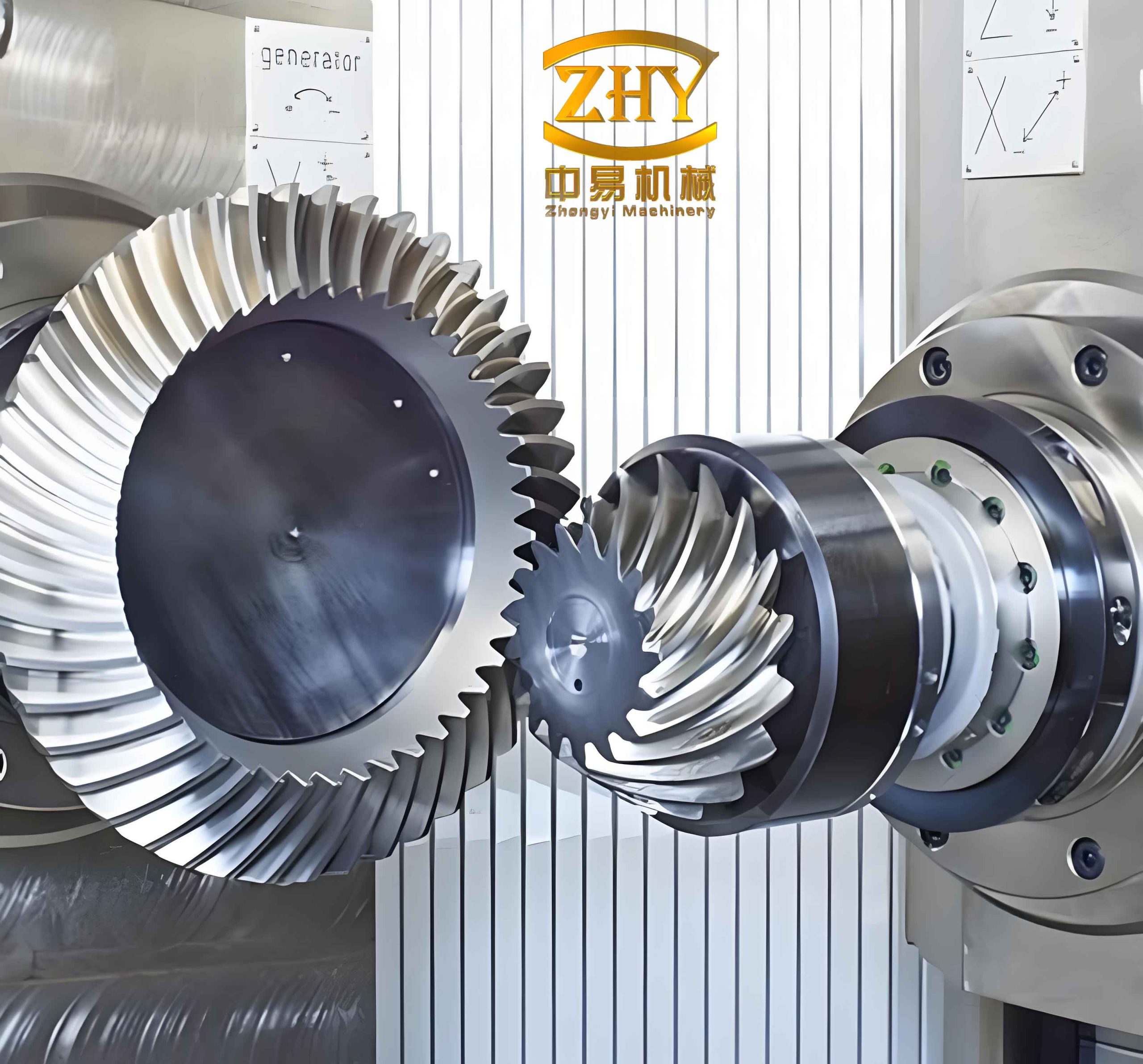
The fundamental goal in designing hyperboloid gears is to control their meshing characteristics precisely. These include locating the contact pattern correctly on the tooth flank to ensure load capacity, controlling the size of the instantaneous contact ellipse, dictating the direction of the contact path relative to the surface principal directions for adequate lubrication, and prescribing a low-amplitude, parabolic function for transmission error to minimize noise and vibrations. The local synthesis method achieves this by working with the differential geometry of the mating surfaces at a chosen reference point, allowing the designer to impose these conditions directly as input parameters.
Fundamental Theory: The Local Synthesis Method
The core of the method lies in analyzing the contact between two surfaces. Consider two surfaces $\Sigma_1$ and $\Sigma_2$ in tangency at a point $M$, with a common unit normal vector $\mathbf{n}$. Let $\mathbf{e}_1$ and $\mathbf{e}_2$ be the principal directions on $\Sigma_1$ at $M$, and $\mathbf{e}_1^*$ and $\mathbf{e}_2^*$ be the principal directions on $\Sigma_2$ at $M$. The angle from $\mathbf{e}_1$ to $\mathbf{e}_1^*$ is denoted by $\sigma$. The fundamental relation for surface contact is given by the following matrix equation:
$$ \begin{bmatrix}
\kappa_1^{(1)} – \kappa_1^{(2)} & 0 & -a \\
0 & \kappa_2^{(1)} – \kappa_2^{(2)} & -b \\
-a & -b & -c
\end{bmatrix} \begin{bmatrix}
\cos\sigma \\
\sin\sigma \\
1
\end{bmatrix} = \mathbf{0} $$
where the coefficients are functions of the kinematics and geometry:
$$ a = \mathbf{v}_r^{(12)} \cdot \mathbf{e}_1, \quad b = \mathbf{v}_r^{(12)} \cdot \mathbf{e}_2, \quad c = (\boldsymbol{\omega}^{(1)} – \boldsymbol{\omega}^{(2)}) \times \mathbf{r} \cdot \mathbf{n}. $$
Here, $\mathbf{v}_r^{(12)}$ is the relative velocity at $M$, $\boldsymbol{\omega}^{(i)}$ are the angular velocities, $\mathbf{r}$ is the position vector, and $\kappa_i^{(j)}$ are the principal curvatures.
In the context of gear generation, the tool surface (cutter) and the generated gear surface are in line contact. For line contact between surfaces $\Sigma_1$ and $\Sigma_2$, the rank of the coefficient matrix in Eq. (1) is less than 3. This condition, along with the known kinematics and curvatures of the generating surface, allows for the determination of the principal curvatures and directions of the generated gear surface at the reference point.
For the operational meshing of the finished pinion and gear, point contact is designed to accommodate misalignments. For point contact, the rank of the matrix is 3, and its determinant must be zero. This yields the equation:
$$ (\kappa_1^{(1)} – \kappa_1^{(2)})(\kappa_2^{(1)} – \kappa_2^{(2)})c – a^2(\kappa_2^{(1)} – \kappa_2^{(2)}) – b^2(\kappa_1^{(1)} – \kappa_1^{(2)}) = 0. $$
If we denote $\eta$ as the angle between the contact path direction $\mathbf{v}_r^{(12)}$ and the principal direction $\mathbf{e}_1$, and given the projections $v_{r1} = \|\mathbf{v}_r^{(12)}\|\cos\eta$ and $v_{r2} = \|\mathbf{v}_r^{(12)}\|\sin\eta$, we have $a = v_{r1}$ and $b = v_{r2}$.
A major advantage of the local synthesis method is the ability to prescribe the contact ellipse size. Given a desired semi-major axis length $a_e$ for the contact ellipse under a specific elastic deformation $\delta$, the following relation is used:
$$ a_e = \left[ \frac{\delta}{(\kappa_1^{(1)} – \kappa_1^{(2)})\cos^2\sigma + (\kappa_2^{(1)} – \kappa_2^{(2)})\sin^2\sigma + (\kappa_1^{(1)} – \kappa_1^{(2)})(\kappa_2^{(1)} – \kappa_2^{(2)})c / \Delta} \right]^{1/2}, $$
where $\Delta = a^2(\kappa_2^{(1)} – \kappa_2^{(2)}) + b^2(\kappa_1^{(1)} – \kappa_1^{(2)})$.
Furthermore, the transmission error curve’s shape, ideally a parabolic function, is controlled by the derivative of the transmission ratio with respect to the pinion rotation angle, denoted as $m_{21}’$. This parameter is directly incorporated into the kinematic coefficients $a$, $b$, and $c$.
Thus, for the point contact design phase, with the gear surface parameters known at $M$, and with prescribed values for $\eta$, $a_e$, and $m_{21}’$, the system of equations from the determinant condition (2), the geometric relations for $a$ and $b$, and the ellipse size equation (3) can be solved for the pinion’s principal curvatures $\kappa_1^{(1)}, \kappa_2^{(1)}$ and the angle $\sigma$. This completes the local synthesis at the reference point for the operational gear pair.
Step-by-Step Design Procedure for Hyperboloid Gears
The complete optimized design process for hyperboloid gears using local synthesis follows a systematic sequence, ensuring the final gear pair possesses the desired contact characteristics.
| Step | Objective | Method / Condition Applied |
|---|---|---|
| 1. Reference Point Selection | Define point M on gear tooth flank. | Specify distance $R_{p}$ from pitch cone apex and offset $z_m$ from tooth centerline. |
| 2. Gear Machine Settings | Define basic gear blank and cutter geometry. | Choose settings (tilt, swivel, etc.) or use standard formulas. Cutter geometry is defined. |
| 3. Gear Tooth Surface $\Sigma_2$ | Determine gear surface geometry at M. | Apply local synthesis for line contact between gear and generating tool. Solve for $\kappa_i^{(2)}, \mathbf{e}_i^{(2)}$. |
| 4. Operational Meshing Synthesis | Define pinion surface geometry at M for desired performance. | Apply local synthesis for point contact between gear and pinion. Input $\eta$, $a_e$, $m_{21}’$. Solve for $\kappa_i^{(1)}, \sigma$. |
| 5. Pinion Machine Settings | Determine pinion cutter and machine settings. | Apply local synthesis for line contact between pinion and its generating tool. Use $\kappa_i^{(1)}$ from Step 4 to solve for machine parameters (vertical offset, axial distance, ratio of roll, etc.). |
Detailed Mathematical Derivation for Hyperboloid Gears
1. Definition of the Reference Point
The reference point $M$ is selected on the gear tooth surface. Its location is defined in the gear axial section by the distance $R_{p}$ from the pitch cone apex $O_p$ along the pitch line and the offset $z_m$ from the tooth centerline at that section. Using the gear’s basic geometry data such as pitch angle $\delta$, root angle $\delta_f$, dedendum angle $\theta_f$, whole depth $h_g$, and dedendum $h_{fg}$, the coordinates of $M$ relative to the gear’s coordinate system can be precisely calculated. This allows full control over where the primary contact zone will be located.
2. Gear Cutting Tool and Surface Generation
The gear is generated using a conical cutter (for Formate or Helixform cycles). The cutter surface $\Sigma_c^g$ is defined in its own coordinate system $S_c^g$ by parameters $\theta_c$ and $u_c$:
$$ \mathbf{r}_c^{(g)}(\theta_c, u_c) = \begin{bmatrix} (R_{c0} + u_c \sin\alpha_c) \cos\theta_c \\ (R_{c0} + u_c \sin\alpha_c) \sin\theta_c \\ -u_c \cos\alpha_c \end{bmatrix}, $$
where $R_{c0}$ is the cutter point radius and $\alpha_c$ is the cutter blade angle.
The coordinate transformation from the cutter to the gear involves the machine settings: machine center to back ($X_{B}$), sliding base ($X_{D}$), blank offset ($E_{m}$), cutter radial setting ($S_{r}$), angular setting ($q$), and the ratio of roll $R_{a}$. The generated gear surface $\Sigma_2$ is the envelope of the family of tool surfaces relative to the gear coordinate system $S_2$. The meshing equation $\mathbf{n}_c^{(g)} \cdot \mathbf{v}_c^{(c2)}=0$ must be satisfied, where $\mathbf{v}_c^{(c2)}$ is the relative velocity between cutter and gear. At the predetermined reference point $M$, solving the system of equations formed by the surface transformation and the meshing equation yields the specific machine kinematics (cutter phase angle $\phi_c$, gear rotation $\phi_2$) for that point. Subsequently, the position vector $\mathbf{r}_M^{(2)}$, unit normal $\mathbf{n}_M^{(2)}$, and principal directions $\mathbf{e}_1^{(2)}, \mathbf{e}_2^{(2)}$ of the gear surface at $M$ are computed. One principal curvature of the gear surface, say $\kappa_1^{(2)}$, is also determined from the generation kinematics.
3. Operational Mesh of Gear and Pinion
The pinion and gear operate with fixed axes defined by the shaft angle $\gamma$ and offset $E$. The coordinate systems $S_1$ (pinion) and $S_2$ (gear) rotate about their axes with angles $\phi_1$ and $\phi_2$, related by the nominal ratio $i_{21} = \phi_2 / \phi_1$. The condition for contact at $M$ is given by the meshing equation in the fixed coordinate system:
$$ \mathbf{n}^{(1)} \cdot \mathbf{v}^{(12)} = 0, $$
where $\mathbf{v}^{(12)}$ is the relative velocity. For the prescribed derivative of the transmission ratio $m_{21}’$, the kinematic coefficients $a, b, c$ in equations (1) and (2) become known functions. As described in the theory section, with $\kappa_1^{(2)}, \kappa_2^{(2)}, \mathbf{e}_1^{(2)}, \mathbf{e}_2^{(2)}$ known from the gear generation, and with designer-specified inputs $\eta$, $a_e$, and $m_{21}’$, the system of equations is solved to obtain the required pinion principal curvatures $\kappa_1^{(1)}, \kappa_2^{(1)}$ and the principal direction angle $\sigma$ at the reference point $M$. This completes the synthesis of the pinion tooth surface geometry needed to achieve the target contact characteristics.
4. Pinion Cutting Tool and Machine Settings Determination
The pinion is generated using its own conical cutter. The cutter surface $\Sigma_c^p$ is defined similarly in system $S_c^p$:
$$ \mathbf{r}_c^{(p)}(\theta_c, u_c) = \begin{bmatrix} (R_{c0} + u_c \sin\alpha_c) \cos\theta_c \\ (R_{c0} + u_c \sin\alpha_c) \sin\theta_c \\ u_c \cos\alpha_c \end{bmatrix}. $$
The pinion machine setup involves parameters like the pinion root angle $\delta_{f1}$, machine root angle $\zeta_1$, initial cradle angle $\phi_{1c0}$, and the key machine settings to be determined: pinion vertical offset $V_{1}$, axial distance $H_1$, and the ratio of roll $R_{a1}$.
The pinion surface $\Sigma_1$ is the envelope of its cutter. The condition for the pinion and gear to be in contact at $M$ with the proper normal vector provides two independent equations to solve for the initial pinion rotation $\phi_{1}^{(0)}$ and a phase angle. More critically, for the pinion generation process, the generated surface $\Sigma_1$ and the cutter surface $\Sigma_c^p$ are in line contact. Therefore, the local synthesis condition for line contact (rank of matrix < 3) is applied. In this scenario, the principal curvatures of the pinion surface $\kappa_1^{(1)}$ and $\kappa_2^{(1)}$ are now known from Step 3. For the conical cutter, one of its principal curvatures at $M$ is zero ($\kappa_{1c}^{(p)}=0$), and the other is a known function of the cutter geometry and instantaneous contact point. The line contact condition from Eq. (1) generates three scalar equations. Combining these with the necessary geometric transformations and the known values, a system of equations is formed. The unknowns solved from this system are the crucial pinion machine settings: the vertical offset $V_{1}$, the axial distance $H_1$, and the ratio of roll $R_{a1}$. Additional settings like the cutter radial position $S_{r1}$ and the basic machine offset $X_{B1}$ can then be derived from geometric relations:
$$ S_{r1} = R_{c1} – R_{c0}, \quad \text{where } R_{c1} \text{ is the computed cutter radius at M}, $$
$$ X_{B1} = H_1 – V_{1} \cot \zeta_1 + \Delta X_1. $$
Here, $\Delta X_1$ is a constant based on the pinion design. This process yields a complete set of machine instructions for cutting the pinion.
Summary of Key Equations for Local Synthesis
The following table consolidates the major equations used in the local synthesis method for hyperboloid gears.
| Phase | Governing Equations | Unknowns / Outputs |
|---|---|---|
| General Contact | $$ \begin{bmatrix} \Delta\kappa_1 & 0 & -a \\ 0 & \Delta\kappa_2 & -b \\ -a & -b & -c \end{bmatrix} \begin{bmatrix} \cos\sigma \\ \sin\sigma \\ 1 \end{bmatrix} = \mathbf{0} $$ where $\Delta\kappa_i = \kappa_i^{(1)} – \kappa_i^{(2)}$. |
Links curvatures, direction angle, and kinematics. |
| Point Contact (Operational Mesh) | 1. Determinant Condition: $(\Delta\kappa_1)(\Delta\kappa_2)c – a^2(\Delta\kappa_2) – b^2(\Delta\kappa_1)=0$ 2. Kinematics: $a=v_{r1}, b=v_{r2}$ 3. Ellipse Size: $a_e = \sqrt{ \delta / \left( \Delta\kappa_1 \cos^2\sigma + \Delta\kappa_2 \sin^2\sigma + (\Delta\kappa_1)(\Delta\kappa_2)c/\Delta \right) }$ |
Solve for $\kappa_1^{(1)}, \kappa_2^{(1)}, \sigma$ given $\eta, a_e, m_{21}’$. |
| Line Contact (Generation) | Rank of coefficient matrix in Eq. (1) is less than 3. Provides equations relating generating tool curvatures to generated gear curvatures. | Solve for unknown gear curvatures (Step 3) or for machine settings $V_1, H_1, R_{a1}$ (Step 5). |
Advantages and Implementation
The local synthesis method transforms the design of hyperboloid gears from an art into a controlled science. The primary advantages are clear. First, it eliminates the extensive trial-and-error cutting, dramatically reducing setup time and cost. Second, it guarantees optimal meshing quality from the first cut, as parameters like contact ellipse size $a_e$, path angle $\eta$, and transmission error slope $m_{21}’$ are direct inputs. This leads to hyperboloid gears with predictable performance: high strength due to controlled contact pattern location, low noise due to optimized transmission error, and good lubrication due to the prescribed contact path direction.
The derivation presented is applicable to machining methods like Gleason’s Helixform or Formate processes. The entire procedure is highly amenable to computerization. A software program implementing this algorithm can calculate all machining parameters for a pair of hyperboloid gears in seconds, requiring only the basic blank data and the desired contact performance specifications as input. While the synthesis is performed at a single reference point, the smoothness of the surfaces ensures the defined characteristics are maintained over a region around that point. For cases involving significant misalignments or deformations that might shift the contact zone away from the designed point, the method can be extended to third-order analysis (including derivatives of curvatures) to make the contact characteristics less sensitive to such shifts, often by incorporating modified roll or cutter tilt.
Conclusion
In summary, the local synthesis method provides a rigorous and efficient mathematical foundation for the optimized machine design of hyperboloid gears. By formulating the problem in terms of differential geometry and kinematic constraints at a reference point, it allows the engineer to directly dictate critical performance attributes. The step-by-step procedure, moving from gear generation to operational mesh synthesis and finally to pinion generation, ensures a closed-form solution for all cutting machine settings. This approach represents a significant advancement over traditional empirical methods, offering precision, reliability, and efficiency in the production of high-performance hyperboloid gears for demanding automotive and industrial applications. The ability to translate desired functional performance directly into manufacturing instructions makes it an indispensable tool in modern gear design and production.