
I treat the parametric modeling of straight bevel gears as a geometry-driven process rather than a sequence of disconnected CAD operations. My objective is to obtain a robust, fully associative model in which every tooth flank, root fillet, and reference plane is controlled by a small set of equations. In this approach, the involute profile and the root transition curve are both generated from symmetric equations, so the tooth space remains balanced about its centerline. This is important for straight bevel gears because a small angular error at the back cone can propagate through the entire tooth solid and produce a visually plausible but dimensionally incorrect gear. By using symmetric equations, I can control the start and end angles of the curves, preserve the design parameters, and rebuild the model after parameter changes without losing the intended tooth form.
The modeling logic I use begins with the standard large-end parameters of straight bevel gears. The large end is taken as the design reference because it normally carries the standard module and pressure angle. Since the spherical involute of a straight bevel gear cannot be developed exactly on a plane, I use the back-cone approximation and study the equivalent cylindrical gear. The tooth profile of this equivalent gear has the same module and pressure angle as the large end of the straight bevel gear, and its equivalent tooth number determines whether the profile is composed only of an involute or of an involute plus a root transition curve. This classification is the first decision point in my modeling workflow.
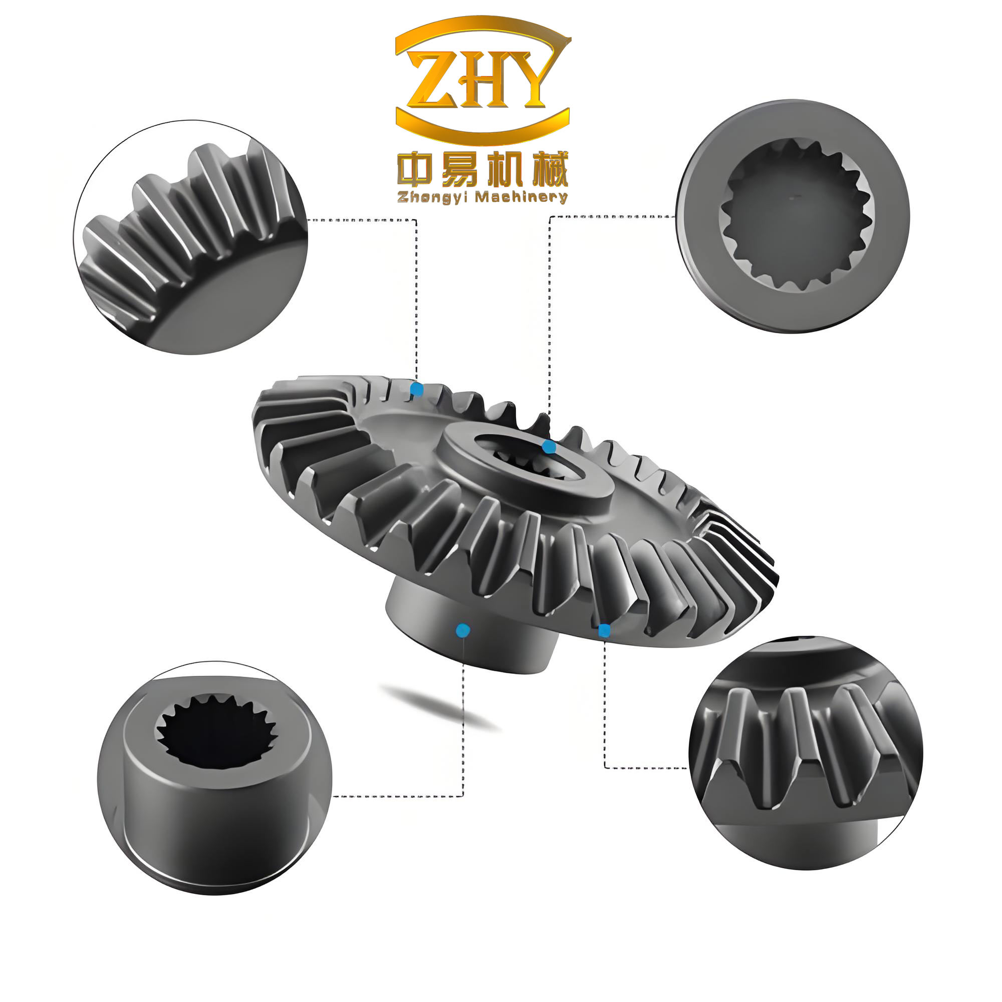
Geometric Basis of Straight Bevel Gears
For straight bevel gears, I define the pitch cone, the back cone, the root cone, and the tip cone as the primary reference surfaces. The pitch cone angle is determined by the gear ratio. In a standard orthogonal pair, the sum of the two pitch cone angles is \(90^\circ\). The equivalent gear is obtained by unfolding the back cone and completing it as a cylinder. This equivalent gear is not a physical part of the straight bevel gear, but it provides a convenient planar representation of the large-end tooth profile.
The basic parameter relations I use are summarized in the following table. These relations are evaluated in the expression system of the CAD environment before any sketch or solid feature is created. Keeping them as named expressions is essential because it allows the same model to represent different straight bevel gears by changing only the primary inputs.
| Quantity | Symbol | Relation | Role in the model |
|---|---|---|---|
| Module | \(m\) | Input | Scales all tooth dimensions |
| Number of teeth | \(z\) | Input | Controls equivalent tooth number and indexing |
| Pressure angle | \(\alpha\) | Input | Controls involute shape and base circle |
| Addendum coefficient | \(h_a^*\) | Input, usually \(1.0\) | Controls addendum height |
| Clearance coefficient | \(c^*\) | Input, usually \(0.2\) | Controls dedendum and root clearance |
| Pitch cone angle | \(\delta\) | \(\delta_1=\arctan(z_1/z_2)\), \(\delta_2=\arctan(z_2/z_1)\) | Defines pitch cone |
| Equivalent tooth number | \(z_v\) | \(z_v=z/\cos\delta\) | Selects profile construction case |
| Pitch diameter | \(d\) | \(d=mz\) | Defines pitch circle at large end |
| Base radius | \(r_b\) | \(r_b=\frac{d}{2}\cos\alpha\) | Defines involute origin |
| Addendum | \(h_a\) | \(h_a=h_a^*m\) | Defines tip cone |
| Dedendum | \(h_f\) | \(h_f=(h_a^*+c^*)m\) | Defines root cone |
| Cone distance | \(R\) | \(R=\frac{m}{2}\sqrt{z_1^2+z_2^2}\) | Defines cone apex location |
| Face width | \(b\) | \(b\le R/3\) | Limits axial tooth length |
| Root angle | \(\delta_f\) | \(\delta_f=\delta-\theta_f\) | Defines root cone |
| Tip angle complement | \(\delta_a’\) | \(\delta_a’=90^\circ-\theta_f\) | Defines equal-clearance tip cone |
The base radius, addendum radius, and root radius are the three radii that control the start and end of the involute. For the equivalent gear, I write them as:
$$r_b=\frac{m z_v}{2}\cos\alpha$$
$$r_a=\frac{m z_v}{2}+h_a^*m$$
$$r_f=\frac{m z_v}{2}-(h_a^*+c^*)m$$
These quantities are evaluated at the large end of the straight bevel gear. The root transition curve is then constructed in the same back-cone plane so that it joins the involute in a controlled manner. I avoid trimming the involute with arbitrary sketch entities because trimming often deletes the parametric relation and introduces asymmetry. Instead, I restrict the domain of the involute parameter itself.
Tooth Profile Classification for Straight Bevel Gears
The equivalent tooth number \(z_v\) determines the lower bound of the usable involute. For a standard involute cylindrical gear, the commonly used boundary equivalent tooth number is \(17\). Therefore, I separate straight bevel gears into two cases. When \(z_v>17\), the tooth profile can be represented by involute curves alone. When \(z_v\le 17\), undercut becomes possible, and the profile must include a root transition curve generated by the cutter tip. This distinction is critical because a straight bevel gear with a small equivalent tooth number cannot be modeled accurately by simply extending the involute to the root circle.
| Case | Condition | Profile composition | Boundary angle source | Modeling consequence |
|---|---|---|---|---|
| I | \(z_v>17\) | Involute only | Root circle or base circle, whichever is larger | No cutter-generated fillet is required |
| II | \(z_v\le 17\) | Involute plus root transition curve | Base circle and transition curve junction | Cutter tip radius must be included |
The equivalent tooth numbers for the two members of a straight bevel gear pair are:
$$z_{v1}=\frac{z_1}{\cos\delta_1}$$
$$z_{v2}=\frac{z_2}{\cos\delta_2}$$
I compute both values and compare them with the boundary value. In a pair, it is possible for one member to fall into Case I and the other into Case II. Therefore, the modeling logic must be applied member by member. I do not assume that both gears of a pair share the same profile composition.
The pressure angle at the addendum and at the root is needed to define the involute range. I use:
$$\alpha_a=\arccos\left(\frac{r_b}{r_a}\right)$$
$$\alpha_f=\arccos\left(\frac{r_b}{r_f}\right)$$
When \(r_f<r_b\), a="" and="" at="" base="" bevel="" by="" cannot="" circle="" circle,="" circle.="" curve="" curve.="" gears="" geometric="" in="" inside="" involute="" involute.
Symmetric Involute Equation
I generate the involute on the back-cone plane using a parametric representation. Let \(u\) be the involute parameter, which is related to the roll angle. The standard involute coordinates are:
$$x_1(u)=r_b(\cos u+u\sin u)$$
$$y_1(u)=r_b(\sin u-u\cos u)$$
Alternatively, I can write the involute in polar form using the involute function:
$$\operatorname{inv}\alpha=\tan\alpha-\alpha$$
$$r(\alpha)=\frac{r_b}{\cos\alpha}$$
For the tooth space, the involute must be mirrored about the centerline of the space. I define the symmetry angle \(\gamma\). For a standard straight bevel gear, I use:
$$\gamma=-\frac{90^\circ}{z_v}+\operatorname{inv}\alpha$$
The first term \(90^\circ/z_v\) represents half of the angular pitch of the equivalent gear. The second term adjusts the position of the involute relative to the tooth centerline. The sign of \(\gamma\) depends on the chosen coordinate orientation. I keep the sign convention consistent throughout the sketch so that the left and right flanks are generated by the same equation set.
For a point \((x_1,y_1)\) on the base involute, the symmetric point \((x_2,y_2)\) about the line inclined at \(\gamma\) is obtained from the point-reflection formula I use in the model:
$$x_2=x_1+\frac{2\sin\gamma\left(y_1-x_1\sin\gamma\right)}{1+\sin^2\gamma}$$
$$y_2=y_1-\frac{2\left(y_1-x_1\sin\gamma\right)}{1+\sin^2\gamma}$$
This formula is implemented directly in the law curve or equation-driven curve feature. It creates the opposite flank without using a non-parametric transform command. As a result, the two flanks remain symmetric when the primary parameters are changed. This is one of the main reasons I prefer symmetric equations for straight bevel gears.
| Involute Entity | Parameter Range | Generated Flank | Symmetry Operation |
|---|---|---|---|
| Base involute \(C_1\) | \(u_{\text{start}}\le u\le u_{\text{end}}\) | Right flank | None |
| Symmetric involute \(C_2\) | Same as \(C_1\) | Left flank | Equation (5) about \(\gamma\) |
| Root transition \(C_3\) | \(\phi_{\text{start}}\le\phi\le\phi_{\text{end}}\) | Right root fillet | None |
| Symmetric root transition \(C_4\) | Same as \(C_3\) | Left root fillet | Equation (5) about \(\gamma\) |
Root Transition Curve for Straight Bevel Gears
For straight bevel gears with \(z_v\le17\), I include the root transition curve generated by the rack cutter tip. This curve does not participate in the meshing action, but it influences the bending fatigue strength and the physical clearance at the root. A model that ignores the transition curve may look acceptable in a rendering, but it will not represent the actual manufactured root shape.
I define the rack cutter tip radius as \(\rho_a\). For a standard full-depth tooth, the fundamental cutter dimensions are:
$$\rho_a=0.38m$$
$$h_a^*=1.0$$
$$c^*=0.2$$
The cutter tip coordinates in its own local system are written as:
$$x_c=\rho_a\sin\phi$$
$$y_c=\rho_a(1-\cos\phi)-h_a^*m$$
Here, \(\phi\) is the local parameter of the cutter tip arc. The transition curve is generated by rolling the cutter pitch line on the pitch circle of the equivalent gear. I use the parameter \(\theta\) for the rolling angle:
$$\theta=\frac{h_a^*m-\rho_a}{\rho_a\sin\phi}$$
The generated transition curve in the gear coordinate system is then represented as:
$$x_t=x_c\cos\theta+y_c\sin\theta+r\left(\theta\sin\theta+\cos\theta\right)$$
$$y_t=x_c\sin\theta-y_c\cos\theta+r\left(\theta\cos\theta-\sin\theta\right)$$
At the junction with the involute, the transition curve must be rotated by a small angle so that the end point and tangent direction are continuous. I define this rotation angle as \(\theta_2\). The rotated coordinates are:
$$x_r=x_t\cos\theta_2+y_t\sin\theta_2$$
$$y_r=-x_t\sin\theta_2+y_t\cos\theta_2$$
The rotation angle \(\theta_2\) is computed from the junction condition. I express it as:
$$\theta_2=\operatorname{inv}\alpha_j-\alpha_j+\theta_j$$
where \(\alpha_j\) is the pressure angle at the junction and \(\theta_j\) is the corresponding rolling parameter. In practice, I solve for \(\theta_2\) numerically or by using the expression list in the CAD system. The important point is that the rotation angle is not chosen by visual inspection; it is determined from the involute and transition curve equations.
After rotation, the transition curve is mirrored about the same symmetry line used for the involute. The symmetric transition curve is:
$$x_{r2}=x_r+\frac{2\sin\gamma\left(y_r-x_r\sin\gamma\right)}{1+\sin^2\gamma}$$
$$y_{r2}=y_r-\frac{2\left(y_r-x_r\sin\gamma\right)}{1+\sin^2\gamma}$$
This produces a balanced root fillet on both sides of the tooth space. A small discontinuity can still appear at the theoretical junction because of numerical tolerance. When this occurs, I insert a short bridge curve with tangent continuity. The bridge curve is not a design feature; it is a numerical closure element. It prevents the solid feature from failing when the tooth space is extruded or ruled.
| Transition Curve Parameter | Meaning | Typical Value or Relation | Effect on Straight Bevel Gears |
|---|---|---|---|
| \(\rho_a\) | Cutter tip radius | \(0.38m\) | Controls fillet size and stress concentration |
| \(\phi\) | Cutter tip arc parameter | Computed range | Defines local fillet shape |
| \(\theta\) | Rolling angle | \(\frac{h_a^*m-\rho_a}{\rho_a\sin\phi}\) | Generates trochoidal motion |
| \(\theta_2\) | Junction rotation | From involute-transition continuity | Aligns fillet with involute |
| \(\gamma\) | Symmetry angle | \(-90^\circ/z_v+\operatorname{inv}\alpha\) | Balances tooth space |
Start and End Angles of the Tooth Profile
The start and end angles of the involute are controlled by the parameter range. I do not draw a long involute and then trim it. Instead, I calculate the angles before the curve is generated. This preserves the parametric nature of the straight bevel gear model and prevents the loss of the symmetric relation.
For \(z_v>17\), the involute can extend to the root circle. Therefore, the starting angle is based on the root pressure angle:
$$\theta_{\text{start}}=\operatorname{inv}\alpha_f\cdot\frac{180^\circ}{\pi}$$
$$\alpha_f=\arccos\left(\frac{r_b}{r_f}\right)$$
For \(z_v\le17\), the involute starts at the base circle because the root circle lies inside the base circle. Thus:
$$\theta_{\text{start}}=\operatorname{inv}\alpha_b\cdot\frac{180^\circ}{\pi}$$
$$\alpha_b=0$$
In practice, I use a very small positive angle at the base circle to avoid a singular tangent. The ending angle is determined by the addendum circle:
$$\theta_{\text{end}}=\operatorname{inv}\alpha_a\cdot\frac{180^\circ}{\pi}$$
$$\alpha_a=\arccos\left(\frac{r_b}{r_a}\right)$$
The involute parameter \(u\) is then mapped linearly from the start angle to the end angle:
$$u(t)=\theta_{\text{start}}+t\left(\theta_{\text{end}}-\theta_{\text{start}}\right)$$
where \(0\le t\le1\). This single parameter \(t\) drives both the right involute and the symmetric left involute. Because the same \(t\) is used for both sides, the two flanks remain synchronized when the model is updated.
| Quantity | Formula | Used When | Purpose |
|---|---|---|---|
| Root pressure angle | \(\alpha_f=\arccos(r_b/r_f)\) | \(z_v>17\) | Start of involute at root |
| Base pressure angle | \(\alpha_b=0\) | \(z_v\le17\) | Start of involute at base circle |
| Addendum pressure angle | \(\alpha_a=\arccos(r_b/r_a)\) | All cases | End of involute at tip |
| Start angle | \(\theta_{\text{start}}=\operatorname{inv}\alpha_{\text{start}}\cdot180^\circ/\pi\) | All cases | First point of involute |
| End angle | \(\theta_{\text{end}}=\operatorname{inv}\alpha_a\cdot180^\circ/\pi\) | All cases | Last point of involute |
| Symmetry angle | \(\gamma=-90^\circ/z_v+\operatorname{inv}\alpha\) | All cases | Mirroring both flanks |
The transition curve has its own start and end parameters. I define the start at the point where the cutter tip begins to generate the fillet and the end at the point where the fillet meets the root circle. The range is chosen so that the transition curve does not intersect the involute. If the two curves overlap, the resulting solid may contain a self-intersection or a zero-thickness region. I check this condition by comparing the junction pressure angle with the involute start angle.
Parameter Definitions for Straight Bevel Gears
I organize the model parameters into three groups: primary parameters, computed parameters, and profile-specific parameters. The primary parameters are the only values that need to be changed when a new straight bevel gear is required. The computed parameters are driven by equations. The profile-specific parameters control the start and end of the curves and the symmetry relation.
| Primary Parameter | Symbol | Example Value | Description |
|---|---|---|---|
| Module | \(m\) | 3 mm | Standard large-end module |
| Pinion tooth number | \(z_1\) | 20 | Number of teeth on pinion |
| Gear tooth number | \(z_2\) | 40 | Number of teeth on gear |
| Pressure angle | \(\alpha\) | 20° | Standard pressure angle |
| Addendum coefficient | \(h_a^*\) | 1.0 | Standard addendum factor |
| Clearance coefficient | \(c^*\) | 0.2 | Standard clearance factor |
| Computed Parameter | Symbol | Formula | Typical Result |
|---|---|---|---|
| Pinion pitch cone angle | \(\delta_1\) | \(\arctan(z_1/z_2)\) | 26.565° |
| Gear pitch cone angle | \(\delta_2\) | \(\arctan(z_2/z_1)\) | 63.435° |
| Pinion equivalent teeth | \(z_{v1}\) | \(z_1/\cos\delta_1\) | 22.36 |
| Gear equivalent teeth | \(z_{v2}\) | \(z_2/\cos\delta_2\) | 89.44 |
| Pitch diameter | \(d\) | \(mz\) | 60 mm, 120 mm |
| Base radius | \(r_b\) | \(d\cos\alpha/2\) | 28.19 mm, 56.38 mm |
| Cone distance | \(R\) | \(\frac{m}{2}\sqrt{z_1^2+z_2^2}\) | 67.08 mm |
| Face width | \(b\) | \(R/3\) | 22.36 mm |
| Addendum | \(h_a\) | \(h_a^*m\) | 3 mm |
| Dedendum | \(h_f\) | \((h_a^*+c^*)m\) | 3.6 mm |
| Profile Parameter | Symbol | Formula or Rule | Purpose |
|---|---|---|---|
| Involute start angle | \(\theta_{\text{start}}\) | Case I or Case II | First point of involute |
| Involute end angle | \(\theta_{\text{end}}\) | \(\operatorname{inv}\alpha_a\cdot180^\circ/\pi\) | Last point at addendum |
| Involute parameter | \(u\) | Linear interpolation | Drives curve generation |
| Symmetry angle | \(\gamma\) | \(-90^\circ/z_v+\operatorname{inv}\alpha\) | Mirrors flanks |
| Cutter tip radius | \(\rho_a\) | \(0.38m\) | Controls root fillet |
| Junction rotation | \(\theta_2\) | From continuity condition | Connects involute and fillet |
Back-Cone Datum Plane and Coordinate System
The back-cone datum plane is the most important reference in my straight bevel gear modeling method. If this plane is incorrectly oriented, the tooth profile will be rotated or scaled incorrectly, and the resulting solid will not match the theoretical straight bevel gear. I construct the back-cone datum plane from the cone geometry rather than from an arbitrary offset plane.
The construction sequence I use is as follows. First, I create the pitch cone and the cone apex. Second, I establish an auxiliary line on the pitch cone surface. Third, I create a plane that contains the apex and is perpendicular to the pitch cone surface at the large end. This plane is the back-cone datum plane. Fourth, I define a datum coordinate system on this plane so that the \(x\)-axis lies along the tooth centerline and the \(y\)-axis is tangent to the back cone. The involute and transition curve equations are then evaluated in this coordinate system.
| Step | Reference Geometry | Action | Result |
|---|---|---|---|
| 1 | Pitch cone and apex | Identify the large-end circle | Back-cone location |
| 2 | Auxiliary line on pitch cone | Create line through apex | Plane definition axis |
| 3 | Point and direction | Create plane perpendicular to pitch cone | Back-cone datum plane |
| 4 | Tooth centerline | Create line at symmetry angle | \(x\)-axis of datum system |
| 5 | Back-cone tangent | Create perpendicular line | \(y\)-axis of datum system |
| 6 | Intersection point | Define origin | Back-cone datum coordinate system |
The symmetry angle \(\gamma\) is used to locate the tooth centerline. I set the auxiliary line at \(-\gamma\) from the pitch cone generator, which ensures that the mirrored involute and the original involute form a balanced tooth space. The origin of the datum coordinate system is placed at the large-end pitch point. This point is common to the pitch circle, the back cone, and the equivalent gear.
After the datum coordinate system is established, I create the law curves. I use the involute equations for the main flank, the symmetric equation for the opposite flank, and the transition curve equations for the root fillet. The curves are then joined at the tip and root to form a closed tooth-space section. I avoid using spline approximations unless a numerical bridge is required at the transition junction.
Solid Generation Strategy for Straight Bevel Gears
I generate the tooth space as a ruled solid between the large-end section and the cone apex. The large-end section is the closed tooth-space curve. The apex is a point. A ruled surface between the apex and the large-end section produces the basic tooth space. This is a natural representation of straight bevel gears because the teeth converge toward the apex. The ruled solid is then subtracted from the gear blank.
The gear blank is created by revolving a trapezoidal profile about the gear axis. The trapezoid is defined by the tip cone, the root cone, the back cone, and the front cone. The blank must include the root cone and the tip cone with the correct angles. I use the equal-clearance tip cone for straight bevel gears so that the clearance remains constant along the tooth width.
| Modeling Stage | Feature Type | Input Geometry | Output |
|---|---|---|---|
| Blank creation | Revolve | Trapezoidal section | Gear blank |
| Tooth-space section | Sketch or law curve | Involute and transition equations | Closed section |
| Tooth-space solid | Ruled surface or loft | Apex and large-end section | Single tooth space |
| Boolean operation | Subtract | Tooth space and blank | One cut tooth space |
| Pattern | Circular pattern | Tooth space feature | All tooth spaces |
| Parameter update | Expression update | Primary parameters | New straight bevel gear |
The circular pattern is driven by the tooth number. The pattern angle is \(360^\circ/z\). I pattern the cut feature rather than the tooth solid. This is more robust because the tooth space geometry is symmetric and the resulting gear has the correct number of teeth. If the profile is generated by symmetric equations, the pattern will produce identical tooth spaces around the entire circumference.
When \(z_v\le17\), I include the root transition curve in the tooth-space section. When \(z_v>17\), I omit the transition curve and let the involute extend to the root circle. The same blank and pattern features are used in both cases. Only the tooth-space curve changes. This modular structure is one of the main advantages of using symmetric equations for straight bevel gears.
Validation and Parameter Control
I validate the model by measuring the pitch diameter, addendum diameter, root diameter, tooth thickness, and cone distance. These measurements are compared with the theoretical values. A small deviation is acceptable due to numerical tolerance, but the deviation should not grow when the model is updated. If the deviation grows, it usually indicates that a curve was trimmed or that a reference plane lost its parametric relation.
| Measured Quantity | Theoretical Formula | Acceptance Criterion | Typical Error Source |
|---|---|---|---|
| Pitch diameter | \(d=mz\) | Less than \(10^{-3}m\) | Sketch constraint |
| Addendum diameter | \(d_a=d+2h_a\) | Less than \(10^{-3}m\) | Tip cone angle |
| Root diameter | \(d_f=d-2h_f\) | Less than \(10^{-3}m\) | Root cone angle |
| Cone distance | \(R=\frac{m}{2}\sqrt{z_1^2+z_2^2}\) | Less than \(10^{-3}m\) | Apex location |
| Tooth thickness | \(\pi m/2\) at pitch circle | Less than \(10^{-3}m\) | Symmetry angle |
| Root fillet continuity | Tangent condition | No visible gap | Junction rotation |
Parameter control is performed through the expression table. I change only the primary parameters. The computed parameters and profile parameters update automatically. For a series of straight bevel gears, I can use a spreadsheet-driven expression table or a part-family table. The same parent model can produce many variants without rebuilding the feature tree.
| Parameter Change | Expected Update | Affected Geometry | Risk if Not Parameterized |
|---|---|---|---|
| Module | All diameters and heights scale | Blank, tooth profile, fillet | Tooth thickness error |
| Tooth number | Pattern count changes | Circular pattern | Missing or overlapping teeth |
| Pressure angle | Involute shape changes | Base circle and flank | Incorrect meshing |
| Cone angle | Back-cone section changes | Equivalent gear | Profile distortion |
| Cutter tip radius | Root fillet changes | Transition curve | Stress concentration error |
Mathematical Summary of the Symmetric Method
The symmetric method can be summarized as a set of equations that define the tooth space. I list the main equations below for reference. They are the core of my parametric modeling approach for straight bevel gears.
$$\delta_1=\arctan\left(\frac{z_1}{z_2}\right),\qquad \delta_2=90^\circ-\delta_1$$
$$z_{v1}=\frac{z_1}{\cos\delta_1},\qquad z_{v2}=\frac{z_2}{\cos\delta_2}$$
$$r_b=\frac{mz_v}{2}\cos\alpha$$
$$r_a=\frac{mz_v}{2}+h_a^*m$$
$$r_f=\frac{mz_v}{2}-(h_a^*+c^*)m$$
$$\operatorname{inv}\alpha=\tan\alpha-\alpha$$
$$\gamma=-\frac{90^\circ}{z_v}+\operatorname{inv}\alpha$$
$$x_1=r_b(\cos u+u\sin u),\qquad y_1=r_b(\sin u-u\cos u)$$
$$x_2=x_1+\frac{2\sin\gamma\left(y_1-x_1\sin\gamma\right)}{1+\sin^2\gamma}$$
$$y_2=y_1-\frac{2\left(y_1-x_1\sin\gamma\right)}{1+\sin^2\gamma}$$
$$x_c=\rho_a\sin\phi,\qquad y_c=\rho_a(1-\cos\phi)-h_a^*m$$
$$\theta=\frac{h_a^*m-\rho_a}{\rho_a\sin\phi}$$
$$x_t=x_c\cos\theta+y_c\sin\theta+r\left(\theta\sin\theta+\cos\theta\right)$$
$$y_t=x_c\sin\theta-y_c\cos\theta+r\left(\theta\cos\theta-\sin\theta\right)$$
$$x_r=x_t\cos\theta_2+y_t\sin\theta_2$$
$$y_r=-x_t\sin\theta_2+y_t\cos\theta_2$$
$$x_{r2}=x_r+\frac{2\sin\gamma\left(y_r-x_r\sin\gamma\right)}{1+\sin^2\gamma}$$
$$y_{r2}=y_r-\frac{2\left(y_r-x_r\sin\gamma\right)}{1+\sin^2\gamma}$$
$$\theta_{\text{start}}=\operatorname{inv}\alpha_{\text{start}}\cdot\frac{180^\circ}{\pi}$$
$$\theta_{\text{end}}=\operatorname{inv}\alpha_a\cdot\frac{180^\circ}{\pi}$$
$$u(t)=\theta_{\text{start}}+t\left(\theta_{\text{end}}-\theta_{\text{start}}\right)$$
These equations are evaluated in a coordinate system attached to the back cone. The resulting curve is closed by adding the tip arc and the root arc. The closed section is used to create the tooth space. The tooth space is then patterned around the gear axis. Because all equations are parametric, the straight bevel gear can be regenerated after any primary parameter change.
Practical Observations
In my experience, the most common failure in straight bevel gear modeling is not the involute itself but the root region. A model may look correct near the pitch circle and still have a root fillet that is too shallow, too deep, or discontinuous. The symmetric transition curve avoids this problem because the fillet is generated from the cutter geometry and mirrored about the same centerline as the involute. I check the junction by measuring the tangent angle at the transition point. If the angle difference is larger than a small tolerance, I adjust the numerical bridge or refine the junction rotation angle.
Another practical issue is the orientation of the back-cone datum plane. If the plane is slightly rotated, the equivalent tooth number appears to change, and the start and end angles become inconsistent. I therefore construct the back-cone plane from the cone apex and the large-end pitch point. I do not use an offset plane from the gear axis, because that method does not guarantee perpendicularity to the pitch cone.
I also recommend keeping the number of independent parameters as small as possible. The primary parameters should be sufficient to define the straight bevel gear. All other values should be computed. This avoids conflicting inputs and makes the model easier to update. The expression table is the single source of truth for the geometry.
| Problem | Symptom | Cause | Correction |
|---|---|---|---|
| Asymmetric tooth space | One flank differs from the other | Manual trim or mirror | Use symmetric equations |
| Root gap | Discontinuity at fillet junction | Incorrect rotation angle | Recalculate \(\theta_2\) or add bridge |
| Profile loss after update | Curve becomes non-parametric | Transform or trim operation | Use equation-driven curves |
| Wrong cone angle | Tooth profile misaligned | Incorrect back-cone plane | Rebuild datum plane from apex |
| Pattern failure | Teeth overlap or disappear | Wrong pattern count or angle | Use \(360^\circ/z\) pattern |
Extension to Parametric Families
Once the base model is correct, I extend it to a family of straight bevel gears. The family table contains the primary parameters for each variant. The CAD system regenerates the model from the equations. Because the tooth profile is driven by symmetric equations, each variant maintains the correct tooth space symmetry. This is much faster than rebuilding the model for every new straight bevel gear.
I can also drive the model from a spreadsheet. The spreadsheet columns correspond to the primary parameters. When a row is selected, the model updates. This is useful for standard gear libraries. The same approach can be used for finite-element analysis, where several variants of straight bevel gears are compared under load.
| Variant | Module \(m\) | Pinion Teeth \(z_1\) | Gear Teeth \(z_2\) | Pressure Angle \(\alpha\) | Equivalent Pinion Teeth \(z_{v1}\) | Profile Case |
|---|---|---|---|---|---|---|
| A | 2 | 18 | 36 | 20° | 20.12 | I |
| B | 3 | 12 | 24 | 20° | 13.42 | II |
| C | 4 | 25 | 50 | 20° | 27.95 | I |
| D | 5 | 10 | 30 | 20° | 10.54 | II |
| E | 2.5 | 30 | 60 | 20° | 33.54 | I |
For each variant, I verify the equivalent tooth number and select the appropriate profile construction. The transition curve is included only when needed. This reduces the modeling complexity for larger straight bevel gears while preserving accuracy for smaller ones. The parametric family can be stored as a template and reused in different projects.
Conclusion
I have presented a symmetric-equation method for the parametric modeling of straight bevel gears. The method begins with the standard large-end parameters and uses the back-cone equivalent gear to represent the tooth profile. The equivalent tooth number determines whether the profile consists of an involute only or an involute plus a root transition curve. The involute is generated from a parametric equation and mirrored about the tooth-space centerline using a symmetry angle. The root transition curve is generated from the cutter tip geometry and rotated to join the involute. The start and end angles are calculated from the pressure angles at the root, base, and addendum circles. The back-cone datum plane and coordinate system are constructed from the cone apex and the large-end pitch point. The tooth space is created as a ruled solid and patterned around the gear axis.
The main advantage of this approach is that it preserves the parametric relations of straight bevel gears. The tooth space remains symmetric after parameter changes, the root fillet is correctly represented, and the model can be updated without rebuilding the feature tree. The method is suitable for standard straight bevel gears, small-tooth-number straight bevel gears, and spreadsheet-driven gear families. It also provides a reliable foundation for finite-element analysis and virtual assembly, because the geometry is controlled by equations rather than by manual sketch edits.
In future work, I plan to extend the symmetric-equation method to spiral bevel gears and hypoid gears, where the tooth trace is curved and the transition curve is more complex. The same principle applies: define the profile from the generating geometry, enforce symmetry about the tooth centerline, and control the curve domain with calculated start and end angles. For straight bevel gears, the method already provides a practical balance between mathematical accuracy and CAD robustness.